Main Content

simsd

Simulate linear models with uncertainty using Monte Carlo method

Description

simsd simulates linear models using the Monte Carlo method. The command performs multiple simulations using different values of the uncertain parameters of the model, and different realizations of additive noise and simulation initial conditions. simsd uses Monte Carlo techniques to generate response uncertainty, whereas sim generates the uncertainty using the Gauss Approximation Formula.

simsd(sys,udata) simulates and plots the response of 10 perturbed realizations of the identified model sys. Simulation input data udata is used to compute the simulated response.

The parameters of the perturbed realizations of sys are consistent with the parameter covariance of the original model, sys. If sys does not contain parameter covariance information, the 10 simulated responses are identical. For information about how the parameter covariance information is used to generate the perturbed models, see Generating Perturbations of Identified Model.

example

simsd(sys,udata,N) simulates and plots the response of N perturbed realizations of the identified model sys.

example

simsd(sys,udata,N,opt) simulates the system response using the simulation behavior specified in the option set opt. Use opt to specify uncertainties in the initial conditions and include the effect of additive disturbances.

The simulated responses are all identical if sys does not contain parameter covariance information, and you do not specify additive noise or covariance values for initial states. You specify these values in the AddNoise and X0Covariance options of opt.

example

y = simsd(___) returns the N simulation results in y as a cell array. No simulated response plot is produced. Use with any of the input argument combinations in the previous syntaxes.

example

[y,y_sd] = simsd(___) also returns the estimated standard deviation y_sd for the simulated response.

example

Examples

collapse all

Load the estimation data.

load iddata1 z1

z1 is an iddata object that stores the input-output estimation data.

Estimate a third-order state-space model.

sys = ssest(z1,3);

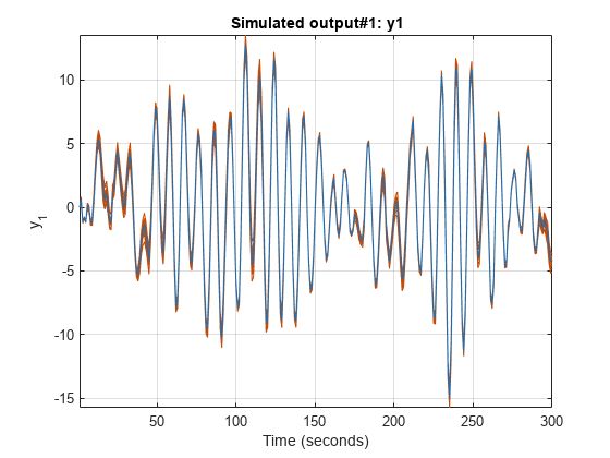
Simulate the response of the estimated model using the Monte Carlo method and input estimation data, and plot the response.

simsd(sys,z1);

Figure Created by subreferencing I/O pairs of a previously estimated model. contains an axes object. The axes object with title Simulated output#1: y1, xlabel Time (seconds), ylabel y indexOf 1 baseline y_1 contains 11 objects of type line. These objects represent y1, Nominal.

The blue line plots the simulated response of the original nominal model sys. The green lines plot the simulated response of 10 perturbed realizations of sys.

Simulate an estimated model using the Monte Carlo method for a specified number of model perturbations.

Estimate a second-order state-space model using estimation data. Obtain sys in the observability canonical form.

load iddata3 z3
sys = ssest(z3,2,'Form','canonical');

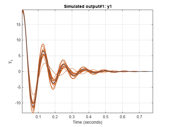
Compute the simulated response of the estimated model using the Monte Carlo method, and plot the responses. Specify the number of random model perturbations as 20.

N = 20;
simsd(sys,z3,N)

Figure Created by subreferencing I/O pairs of a previously estimated model. contains an axes object. The axes object with title Simulated output#1: y1, xlabel Time (seconds), ylabel y indexOf 1 baseline y_1 contains 21 objects of type line. These objects represent y1, Nominal.

The blue line plots the simulated response of the original nominal model sys. The green lines plot the simulated response of the 20 perturbed realizations of sys.

You can also obtain the simulated response for each perturbation of sys. No plot is generated when you use this syntax.

y = simsd(sys,z3,N);

y is the simulated response, returned as a cell array of N+1 elements. y{1} contains the nominal response for sys. The remaining elements contain the simulated response for the N perturbed realizations.

Load time series data.

load iddata9 z9

z9 is an iddata object with 200 output data samples and no inputs.

Estimate a sixth-order AR model using the least-squares algorithm.

sys = ar(z9,6,'ls');

For time series data, specify the desired simulation length, Ns = 200 using an Ns-by-0 input data set.

data = iddata([],zeros(200,0),z9.Ts);

Set the initial conditions to use the initial samples of the time series as historical output samples. The past data is mapped to the initial states of each perturbed system individually.

IC = struct('Input',[],'Output',z9.y(1:6));
opt = simsdOptions('InitialCondition',IC);

Simulate the model using Monte Carlo method and specified initial conditions. Specify the number of random model perturbations as 20.

simsd(sys,data,20,opt)

Figure Created by subreferencing I/O pairs of a previously estimated model. contains an axes object. The axes object with title Simulated output#1: y1, xlabel Time (seconds), ylabel y indexOf 1 baseline y_1 contains 21 objects of type line. These objects represent y1, Nominal.

The blue line plots the simulated response of the original nominal model sys. The green lines plot the simulated response of the 20 perturbed realizations of sys.

Load data, and split it into estimation and simulation data.

load iddata3
ze = z3(1:200);
zsim = z3(201:256);

Estimate a second-order state-space model sys using estimation data. Specify that no parameter covariance data is generated. Obtain sys in the observability canonical form.

opt = ssestOptions('EstimateCovariance',false);
sys = ssest(ze,2,'Form','canonical',opt);

Set the initial conditions for simulating the estimated model. Specify initial state values x0 for the two states and also the covariance of initial state values x0Cov. The covariance is specified as a 2-by-2 matrix because there are two states.

x0 = [1.2; -2.4];
x0Cov = [0.86 -0.39; -0.39 1.42];
opt = simsdOptions('InitialCondition',x0,'X0Covariance',x0Cov);

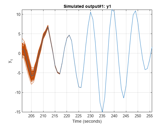
Simulate the model using Monte Carlo method and specified initial conditions. Specify the number of random model perturbations as 100.

simsd(sys,zsim,100,opt)

Figure Created by subreferencing I/O pairs of a previously estimated model. contains an axes object. The axes object with title Simulated output#1: y1, xlabel Time (seconds), ylabel y indexOf 1 baseline y_1 contains 101 objects of type line. These objects represent y1, Nominal.

The blue line plots the simulated response of the original nominal model sys. The green lines plot the simulated response of the 100 perturbed realizations of sys. The software uses a different realization of the initial states to simulate each perturbed model. Initial states are drawn from a Gaussian distribution with mean InitialCondition and covariance X0Covariance.

Load the estimation data.

load iddata1 z1

z1 is an idddata object that stores 300 input-output estimation data samples.

Estimate a second-order state-space model using the estimation data.

sys = ssest(z1,2);

Create a default option set for simsd, and modify the option set to add noise.

opt = simsdOptions;
opt.AddNoise = true;

Compute the simulated response of the estimated model using the Monte Carlo method. Specify the number of random model perturbations as 20, and simulate the model using the specified option set.

[y,y_sd] = simsd(sys,z1,20,opt);

y is the simulated response, returned as a cell array of 21 elements. y{1} contains the nominal, noise-free response for sys. The remaining elements contain the simulated response for the 20 perturbed realizations of sys with additive disturbances added to each response.

y_sd is the estimated standard deviation of simulated response, returned as an iddata object with no inputs. The standard deviations are computed from the 21 simulated outputs. To access the standard deviation, use y_sd.OutputData.

Input Arguments

collapse all

Model to be simulated, specified as one of the following parametric linear identified models: idtf, idproc, idpoly, idss, or idgrey.

To generate the set of simulated responses, the software perturbs the parameters of sys in a way that is consistent with the parameter covariance information. Use getcov to examine the parameter uncertainty for sys. For information about how the perturbed models are generated from sys, see rsample.

The simulated responses are all identical if sys does not contain parameter covariance information and you do not specify additive noise or covariance values for initial states. You specify these values in the AddNoise and X0Covariance options of opt.

Simulation input data, specified as one of the following:

  • iddata object — Input data can be either time-domain or frequency-domain. The software uses only the input channels of the iddata object.

    If sys is a time series model, that is, a model with no inputs, specify udata as an Ns-by-0 signal, where Ns is the wanted number of simulation output samples for each of the N perturbed realizations of sys. For example, to simulate 100 output samples, specify udata as follows.

    udata = iddata([],zeros(100,0),Ts);

    For an example, see Simulate Time Series Model Using Monte Carlo Method.

  • matrix — For simulation of discrete-time systems using time-domain data only. Columns of the matrix correspond to each input channel.

If you do not have data from an experiment, use idinput to generate signals with various characteristics.

Number of perturbed realizations of sys to be simulated, specified as a positive integer.

Simulation options for simulating models using Monte Carlo methods, specified as a simsdOptions option set. You can use this option set to specify:

  • Input and output signal offsets — Specify an offset to remove from the input signal and an offset to add to the response of sys.

  • Initial condition handling — Specify initial conditions for simulation and their covariance. For state-space and linear grey-box models (idss and idgrey), if you want to simulate the effect of uncertainty in initial states, set the InitialCondition option to a double vector, and specify its covariance using the X0Covariance option. For an example, see Study Effect of Initial Condition Uncertainty on Model Response.

  • Addition of noise to simulated data — If you want to include the influence of additive disturbances, specify the AddNoise option as true. For an example, see Study Effect of Additive Disturbance on Response Uncertainty.

Output Arguments

collapse all

Simulated response, returned as a cell array of N+1 elements. y{1} contains the nominal response for sys. The remaining elements contain the simulated response for the N perturbed realizations.

The command performs multiple simulations using different values of the uncertain parameters of the model, and different realizations of additive noise and simulation initial conditions. Thus, the simulated responses are all identical if sys does not contain parameter covariance information and you do not specify additive noise and covariance values for initial states in opt.

Estimated standard deviation of simulated response, returned as an iddata object. The standard deviation is computed as the sample standard deviation of the y ensemble:

y_sd=1Ni=2N+1(y{1}y{i})2

Here y{1} is the nominal response for sys, and y{i} (i = 2:N+1) are the simulated responses for the N perturbed realizations of sys.

More About

collapse all

Generating Perturbations of Identified Model

The software generates N perturbations of the identified model sys and then simulates the response of each of these perturbations. The parameters of the perturbed realizations of sys are consistent with the parameter covariance of the original model sys. The parameter covariance of sys gives information about the distribution of the parameters. However, for some parameter values, the resulting perturbed systems can be unstable. To reduce the probability of generation of unrealistic systems, the software prescales the parameter covariance.

If Δp is the parameter covariance for the parameters p of sys, then the simulated output f(p+Δp) of a perturbed model as a first-order approximation is:

f(p+Δp)=f(p)+fpΔp

The simsd command first scales Δp by a scaling factor s (approximately 0.1%) to generate perturbed systems with parameters (p+sΔp). The command then computes f(p+sΔp), the simulated response of these perturbed systems. Where,

f(p+sΔp)=f(p)+sfpΔp

The command then computes the simulated response f(p+Δp) as:

f(p+Δp)=f(p)+1s(f(p+sΔp)f(p))

Note

This scaling is not applied to the free delays of idproc or idtf models.

If you specify the AddNoise option of simsdOptions as true, the software adds different realizations of the noise sequence to the noise-free responses of the perturbed system. The realizations of the noise sequence are consistent with the noise component of the model.

For state-space models, if you specify the covariance of initial state values in X0Covariance option of simsdOptions, different realizations of the initial states are used to simulate each perturbed model. Initial states are drawn from a Gaussian distribution with mean InitialCondition and covariance X0Covariance.

Version History

Introduced before R2006a