sim

Load the estimation data.

load sdata2 tt2

Estimate a third-order state-space model.

sys = ssest(tt2,3);

Simulate the identified model using the input channels from the estimation data.

y = sim(sys,tt2);

Load the data, and obtain the identified model.

load sdata2 tt2
sys = n4sid(tt2,3);

sys is a third-order state-space model estimated using a subspace method.

Create a simulation option set to add noise to the simulated model response.

opt1 = simOptions('AddNoise',true);

Simulate the model.

y = sim(sys,tt2,opt1);

Default Gaussian white noise is filtered by the noise transfer function of the model and added to the simulated model response.

You can also add your own noise signal, e, using the NoiseData option.

e = randn(length(tt2.u),1);
opt2 = simOptions('AddNoise',true,'NoiseData',e);

Simulate the model.

y = sim(sys,tt2,opt2);

Load the data.

load sdata1 umat1 ymat1 Ts

Specify the estimation option to estimate the initial state.

estimOpt = ssestOptions('InitialState','estimate');

Estimate a state-space model, and return the value of the estimated initial state.

[sys,x0] = ssest(umat1,ymat1,2,'Ts',Ts,estimOpt);

Specify initial conditions for simulation.

simOpt = simOptions('InitialCondition',x0);

Simulate the model, and obtain the model response and standard deviation.

[y,y_sd] = sim(sys,umat1,simOpt);

Load estimation data, and estimate a state-space model.

load iddata1 z1
sys = ssest(z1,2);

Return the standard deviation and state trajectory.

[y,y_sd,x] = sim(sys,z1);

Load estimation data, and estimate a state-space model.

load sdata1 umat1 ymat1 Ts
sys = ssest(umat1,ymat1,2,'Ts',Ts);

Create a simulation option set, and specify the initial states.

opt = simOptions('InitialCondition',[1;2]);

Specify the covariance of the initial states.

opt.X0Covariance = [0.1 0; 0 0.1];

Calculate the standard deviations of simulated response, y_sd, and state trajectory, x_sd.

[y,y_sd,x,x_sd] = sim(sys,umat1,opt);

Obtain the identified model.

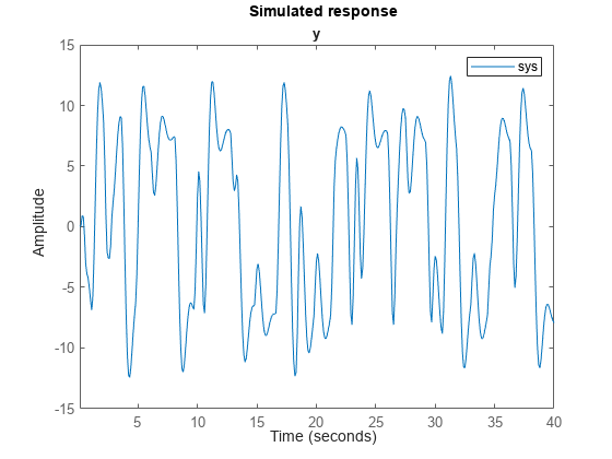
load sdata2 tt2
sys = tfest(tt2,3);

sys is an idtf model that encapsulates the third-order transfer function estimated for the measured data tt2.

Simulate the model.

sim(sys,tt2)

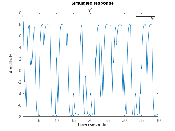
Simulate a single-input single-output nonlinear ARX model around a known equilibrium point, with an input level of 1 and output level of 10.

Load the sample data.

load iddata2

Estimate a nonlinear ARX model from the data.

M = nlarx(z2,[2 2 1],'idTreePartition');

Estimate current states of model based on past data. Specify as many past samples as there are lags in the input and output variables (2 here).

x0 = data2state(M,struct('Input',ones(2,1),'Output',10*ones(2,1)));

Simulate the model using the initial states returned by data2state.

opt = simOptions('InitialCondition',x0);
sim(M,z2,opt)

Continue the simulation of a nonlinear ARX model from the end of a previous simulation run.

Estimate a nonlinear ARX model from data.

load iddata2
M = nlarx(z2,[2 2 1],idTreePartition);

Simulate the model using the first half of the input data z2. Start the simulation from zero initial states.

u1 = z2(1:200,[]); 
opt1 = simOptions('InitialCondition','zero');
ys1 = sim(M,u1,opt1);

Start another simulation using the second half of the input data z2. Use the same states of the model from the end of the first simulation.

u2 = z2(201:end,[]);

To set the initial states for the second simulation correctly, package input u1 and output ys1 from the first simulation into one iddata object. Pass this data as initial conditions for the next simulation.

firstSimData = [ys1,u1];
opt2 = simOptions('InitialCondition',firstSimData);
ys2 = sim(M,u2,opt2);

Verify the two simulations by comparing to a complete simulation using all the input data z2. First, extract the whole set of input data.

uTotal = z2(:,[]); 
opt3 = simOptions('InitialCondition','zero'); 
ysTotal = sim(M,uTotal,opt3);

Plot the three responses ys1, ys2 and ysTotal. ys1 should be equal to first half of ysTotal. ys2 should be equal to the second half of ysTotal.

plot(ys1,'b',ys2,'g',ysTotal,'k*')

The plot shows that the three responses ys1, ys2, and ysTotal overlap as expected.

Estimate initial states of model M such that, the response best matches the output in data set z2.

Load the sample data.

load iddata2;

Estimate a nonlinear ARX model from the data.

M = nlarx(z2,[4 3 2],idWaveletNetwork('NumberOfUnits',20));

Estimate the initial states of M to best fit z2.y in the simulated response.

x0 = findstates(M,z2,Inf);

Simulate the model.

opt = simOptions('InitialCondition',x0);
ysim = sim(M,z2.u,opt);

Compare the simulated model output ysim with the output signal in z2.

time = z2.SamplingInstants;
plot(time,ysim,time,z2.y,'.')

Start simulation of a model near steady state, where the input is known to be 1, but the output is unknown.

Load the sample data.

load iddata2

Estimate a nonlinear ARX model from the data.

M = nlarx(z2,[4 3 2],idWaveletNetwork);

Determine equilibrium state values for input 1 and unknown target output.

x0 = findop(M,'steady',1, NaN);

Simulate the model using initial states x0.

opt = simOptions('InitialCondition',x0);
sim(M,z2.u,opt)

Load the sample data.

load iddata2

Create a Hammerstein-Wiener model.

M = nlhw(z2,[4 3 2],[],idPiecewiseLinear);

Compute steady-state operating point values corresponding to an input level of 1 and an unknown output level.

x0 = findop(M,'steady',1,NaN);

Simulate the model using the estimated initial states.

opt = simOptions('InitialCondition',x0);
sim(M,z2.u)

Load time series data, and estimate an AR model using the least-squares approach.

load iddata9 z9
sys = ar(z9,6,'ls');

For time series data, specify the desired simulation length, N = 200 using an N-by-0 input data set.

data = iddata([],zeros(200,0),z9.Ts);

Set the initial conditions to use the initial samples of the time series as historical output samples.

IC = struct('Input',[],'Output',z9.y(1:6));
opt = simOptions('InitialCondition',IC);

Simulate the model.

sim(sys,data,opt)

Use historical input-output data as a proxy for initial conditions when simulating your model. You first simulate using the sim command and specify the historical data using the simOptions option set. You then reproduce the simulated output by manually mapping the historical data to initial states.

Load a two-input, one-output data set.

load iddata7 z7

Identify a fifth-order state-space model using the data.

sys = n4sid(z7,5);

Split the data set into two parts.

zA = z7(1:15);
zB = z7(16:end);

Simulate the model using the input signal in zB.

uSim = zB;

Simulation requires initial conditions. The signal values in zA are the historical data, that is, they are the input and output values for the time immediately preceding data in zB. Use zA as a proxy for the required initial conditions.

IO = struct('Input',zA.InputData,'Output',zA.OutputData);
opt = simOptions('InitialCondition',IO);

Simulate the model.

ysim = sim(sys,uSim,opt);

Now reproduce the output by manually mapping the historical data to initial states of sys. To do so, use the data2state command.

xf = data2state(sys,zA);

xf contains the state values of sys at the time instant immediately after the most recent data sample in zA.

Simulate the system using xf as the initial states.

opt2 = simOptions('InitialCondition',xf);
ysim2 = sim(sys,uSim,opt2);

Plot the output of the sim command ysim and the manually computed results ysim2.

plot(ysim,'b',ysim2,'--r')

ysim2 is the same as ysim.

The state and output networks of an idNeuralStateSpace object are initialized randomly. To ensure reproducibility, fix the seed of the random number generator.

rng(0)

Create a continuous-time neural state-space object with two states, two inputs, and three outputs.

nss = idNeuralStateSpace(2,NumInputs=2,NumOutputs=3)

nss =

Continuous-time Neural State-Space Model with 3 outputs, 2 states, and 2 inputs
     dx/dt = f(x(t),u(t))
    y_1(t) = x(t) + e_1(t)
    y_2(t) = g(x(t),u(t)) + e_2(t)
      y(t) = [y_1(t); y_2(t)]
 
f(.) network:
  Deep network with 2 fully connected, hidden layers
  Activation function: tanh
g(.) network:
  Deep network with 2 fully connected, hidden layers
  Activation function: tanh
 
Inputs: u1, u2
Outputs: y1, y2, y3
States: x1, x2
 
Status:                                                         
Created by direct construction or transformation. Not estimated.

Define a time sequence, a random input signal, and a random initial state.

t = (0:1:10)';
u = rand(length(t),2);
x0 = 0.3*randn(2,1);

When simulating idNeuralStateSpace systems, specifying input data as a numerical array is not supported. For this example, convert the input data to a timetable object, specifying that the values of u are associated with the time points in the vector t.

u = array2timetable(u,RowTimes=seconds(t));

Set up a simulation options object so that the simulation starts from x0 and the output is calculated for the time points in the vector t.

simOpt = simOptions('InitialCondition',x0,'OutputTimes',t);

Simulate the (untrained) neural state-space system nss.

y = sim(nss,u,simOpt);

Plot the simulated outputs.

plot(t,y.Variables);
ylabel("Outputs"); 
xlabel("Time (seconds)")
title("Neural state-space system: simulated output")