Apply Initial Conditions When Simulating Identified Linear Models

Open Live Script

This example shows the workflow for obtaining and using estimated initial conditions when you simulate models to validate model performance against measured data.

Use initial conditions (ICs) when you want to simulate a model in order to validate model performance by comparing the simulated response to measured data. If your measurement data corresponds to a system that does not start at rest, a simulation that assumes a resting start point results in a mismatch. The simulated and measured responses do not agree at the beginning of the simulation.

For state-space models, the initial state vector is sufficient to describe initial conditions. For other LTI models, the initialCondition object allows you to represent ICs in the form of the free response of your model to the initial conditions. This representation is in state-space form, as shown in the following equation:

$G (s) = C {(sI - A)}_{}^{- 1} X0$

Here, $G (s)$ is the free response that the initialCondition encapsulates. $A$ and $C$ are the A and C matrices of the state-space form of your model. $X0$ is the corresponding initial state vector. The free response does not include B and D matrices because the IC free response is independent of input signals. Although the initialCondition object packages the state-space form, you can use the information to model a free response for any LTI system. The simulation software computes the free and forced responses separately and then adds them together to obtain the total response.

Prepare Data

Load the data and split it into estimation and validation data sets. For this example, the splits occur where the output data has a visibly nonzero start point.

load iddata2 z2
z2e = z2(10:210);
z2v = z2(210:400);
plot(z2e,z2v)

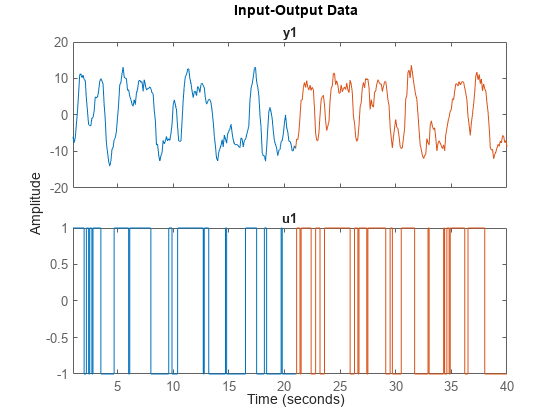
Figure contains 2 axes objects. Axes object 1 with title y1 contains 2 objects of type line. These objects represent z2e, z2v. Axes object 2 with title u1 contains 2 objects of type line. These objects represent z2e, z2v.

Display the first output sample for each data set.

z2e.y(1)

ans = 
-5.9588

z2v.y(1)

ans = 
-9.2141

Estimate Transfer Function Model

Using the estimation data, estimate a second-order transfer function model and return the initial condition ic. Display ic.

np = 2;
nz = 1;
[sys_tf,ic] = tfest(z2e,np,nz);
ic

ic = 
  initialCondition with properties:

     A: [2x2 double]
    X0: [2x1 double]
     C: [-1.6158 5.1969]
    Ts: 0

ic represents the free response of the transfer function model, in state-space form, to the initial condition.

A = ic.A

A = 2×2

   -3.4145   -5.6635
    4.0000         0

C = ic.C

C = 1×2

   -1.6158    5.1969

The X0 property contains the initial state vector.

X0 = ic.X0

X0 = 2×1

   -0.5053
   -1.2941

Simulate Model

Simulate the model. First, as a reference, simulate the model without incorporating ic. Plot the simulated response with the estimation data.

y_no_ic = sim(sys_tf,z2e);
plot(y_no_ic,z2e)
legend('Model Response','Output Data')
title('Transfer Function Model - No IC Specification')

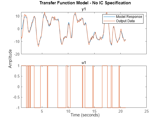
Figure contains 2 axes objects. Axes object 1 with title y1 contains 2 objects of type line. These objects represent Model Response, Output Data. Axes object 2 with title u1 contains an object of type line. This object represents Output Data.

The simulated and measured responses do not agree at the start of the simulation.

Incorporate ic. To do so, first initialize opt to the option set simOptions. Specify ic as the 'InitialCondition' setting. Simulate the model and plot the results.

opt = simOptions;
opt.InitialCondition = ic;
y_ic = sim(sys_tf,z2e,opt);
plot(y_ic,z2e)
legend('Model Response','Output Data')
title('Transfer Function Model - ICs Specified')

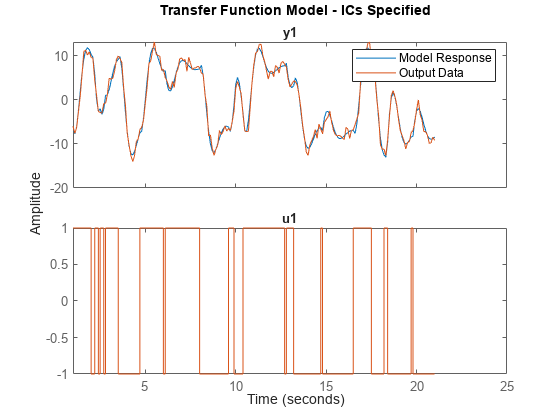
The responses now agree more closely at the start of the simulation.

Obtain ICs for Validation Data

ic represents the ICs only for the estimation data set. If you want to run a simulation using the validation inputs and compare the results with the validation output, you must obtain the ICs for the validation data set. To do so, use compare. You can use compare to estimate ICs for any combination of model and measurement data.

[yv,fitv,icv] = compare(z2v,sys_tf);
icv

icv = 
  initialCondition with properties:

     A: [2x2 double]
    X0: [2x1 double]
     C: [-1.6158 5.1969]
    Ts: 0

Display the A, C, and X0 properties of icv.

Av = icv.A

Av = 2×2

   -3.4145   -5.6635
    4.0000         0

Cv = icv.C

Cv = 1×2

   -1.6158    5.1969

X0v = icv.X0

X0v = 2×1

    0.4512
   -1.5068

For this case, the A and C matrices representing the free-response model are identical to the ic.A and ic.C values in the original estimation. However, the initial state vector X0v is different from ic.X0.

Specify icv as the 'InitialCondition' setting in opt and simulate the model using the validation data. Plot the simulated and measured responses.

opt.InitialCondition = icv;
y_ic = sim(sys_tf,z2v,opt);
plot(y_ic(:,:,[]),z2v(:,:,[]))
legend('Model Response','Output Data')
title('Transfer Function Model Response For Validation Data')

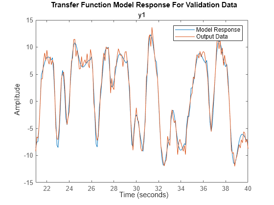
Figure contains an axes object. The axes object with title y1 contains 2 objects of type line. These objects represent Model Response, Output Data.

The simulated and measured responses have good agreement at the start of the simulation.

Apply ICs to Simulation of Converted Model

You can apply the ICs when you convert your model to another form.

Convert sys_tf to an idpoly model. Simulate the converted model, preserving the current SimOptions 'InitialCondition' setting, icv, in opt.

sys_poly = idpoly(sys_tf);
y_poly = sim(sys_poly,z2v,opt);
plot(y_poly(:,:,[]),y_ic(:,:,[]),z2v(:,:,[]))
legend('idpoly Model Response','idtf Model Response','Output Data')
title('Converted Polynomial Model')

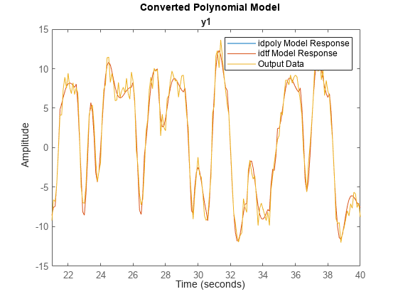
Figure contains an axes object. The axes object with title y1 contains 3 objects of type line. These objects represent idpoly Model Response, idtf Model Response, Output Data.

The sys_tf and sys_poly responses appear identical.

Apply ICs to Simulation of State-Space Model

State-space models can use initial conditions represented either by a single numeric initial state vector or by an initialCondition object.

When you convert sys_tf to an idss model, you can again use icv by retaining the icv setting in opt.

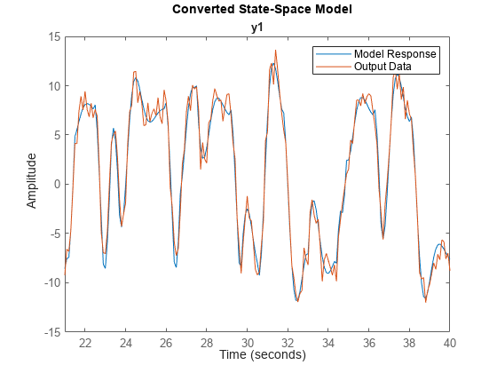
sys_ss = idss(sys_tf);
y_ss = sim(sys_ss,z2v,opt);
plot(y_ss(:,:,[]),z2v(:,:,[]))
legend('Model Response','Output Data')
title('Converted State-Space Model')

Figure contains an axes object. The axes object with title y1 contains 2 objects of type line. These objects represent Model Response, Output Data.

When you use compare or a state-space estimation function such as ssest, the function returns the initial state vector x0. Estimate the state-space model sys_ss2 using z2e and use compare to obtain ICs corresponding to z2v.

sys_ss2 = ssest(z2e,2);
[yvss,fitvss,x0] = compare(z2v,sys_ss2);
x0

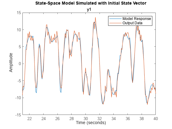
x0 is a numeric vector. Specify x0 as the 'InitialCondition' setting in opt and simulate the response.

opt.InitialCondition = x0;
y_ss2 = sim(sys_ss2,z2v,opt);
plot(y_ss2(:,:,[]),z2v(:,:,[]))
legend('Model Response','Output Data')
title('State-Space Model Simulated with Initial State Vector')

Figure contains an axes object. The axes object with title y1 contains 2 objects of type line. These objects represent Model Response, Output Data.

Convert State-Space Initial State Vector to `initialCondition` Object

If your original model is a state-space model and you want to convert the model into a polynomial or transfer function model and apply the same initial conditions, you must convert the initial state vector into an initialCondition object.

Extract and display the A, C, and Ts properties from sys_ss2.

As = sys_ss2.A

As = 2×2

   -1.7643   -3.7716
    5.2918   -1.7327

Cs = sys_ss2.C

Cs = 1×2

   82.9765   25.5146

Tss = sys_ss2.Ts

Tss = 
0

The A and C matrices that are estimated using ssest have different values than the A and C matrices estimated in icv using tfest. There are infinitely many state-space representations of a given linear model. The two pairs of matrices, along with the associated initial state vectors, are equivalent and produce the same free response.

Create the initialCondition object ic_ss2 using sys_ss2 model properties and the initial state vector x0 you obtained when you used compare.

ic_ss2 = initialCondition(As,x0,Cs,Tss)

ic_ss2 = 
  initialCondition with properties:

     A: [2x2 double]
    X0: [2x1 double]
     C: [82.9765 25.5146]
    Ts: 0

Convert sys_ss2 into a transfer function model and simulate the converted model using ic_ss2 as the 'InitialCondition' setting.

sys_tf2 = idtf(sys_ss2);
opt.InitialCondition = ic_ss2;
y_tf2 = sim(sys_tf2,z2v,opt);
plot(y_tf2(:,:,[]),z2v(:,:,[]))
legend('Model Response','Output Data')
title('Transfer Function Model Converted from State-Space Model')

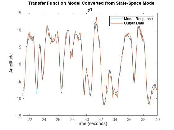
Figure contains an axes object. The axes object with title y1 contains 2 objects of type line. These objects represent Model Response, Output Data.

Using the constructed initialCondition object ic_ss2 produces a similar response to simulated responses that use directly estimated initialCondition objects.

Apply Initial Conditions When Simulating Identified Linear Models

Prepare Data

Estimate Transfer Function Model

Simulate Model

Obtain ICs for Validation Data

Apply ICs to Simulation of Converted Model

Apply ICs to Simulation of State-Space Model

Convert State-Space Initial State Vector to `initialCondition` Object

See Also

Related Topics

Apply Initial Conditions When Simulating Identified Linear Models

Prepare Data

Estimate Transfer Function Model

Simulate Model

Obtain ICs for Validation Data

Apply ICs to Simulation of Converted Model

Apply ICs to Simulation of State-Space Model

Convert State-Space Initial State Vector to initialCondition Object

See Also

Related Topics

Convert State-Space Initial State Vector to `initialCondition` Object