Train and Simulate Simple NARX Network
R2026bThis example trains a nonlinear autoregressive with exogenous inputs (NARX) neural network using both narxnet (Deep Learning Toolbox) and nlarx, and compares its response to the test data output by simulating the trained (open-loop) model in closed-loop. For more information on estimating NARX networks using narxnet and nlarx, see Train NARX Networks Using idnlarx Instead of narxnet.
narxnet Approach
Load the simple time series prediction data.
[X,T] = simpleseries_dataset;
Partition the data into training data XTrain and TTrain, and data for prediction XPredict. Use XPredict to perform prediction after you create the closed-loop network.
% training data
XTrain = X(1:80);
TTrain = T(1:80);

% test data
XPredict = X(81:100);
YPredict = T(81:100);
rng default % for reproducibility of shown results
Create a NARX network using narxnet (Deep Learning Toolbox). Define the input delays, feedback delays, and size of the hidden layers.
numUnits = 4;
model_narxnetOL = narxnet(1:2,1:2,numUnits);
Prepare the time series training data using preparets (Deep Learning Toolbox). This function automatically shifts the input and target time series by the number of steps needed to fill the initial input and layer delay states.
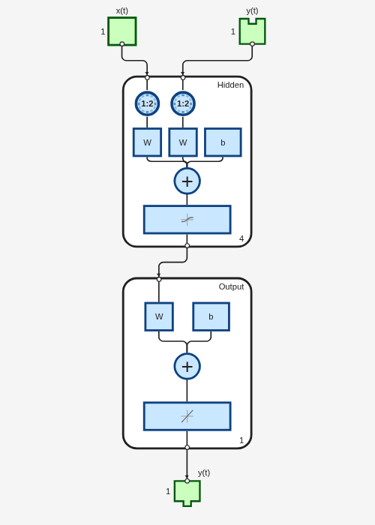
[Xs,Xi,Ai,Ts] = preparets(model_narxnetOL,XTrain,{},TTrain);Train the NARX network and display the trained model. The train (Deep Learning Toolbox) function trains the network in an open-loop, including the validation and testing steps.
model_narxnetOL = train(model_narxnetOL,Xs,Ts,Xi,Ai);
view(model_narxnetOL)
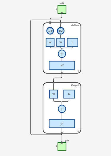
Simulate the model in closed-loop. Since model_narxnet is an open-loop model, first convert it into a closed-loop model using closeloop (Deep Learning Toolbox). Notice the feedback loop in the displayed model.
[model_narxnetCL1,Xi_CL,Ai_CL] = closeloop(model_narxnetOL,Xi,Ai);
view(model_narxnetCL1)
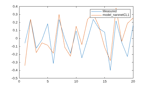
Simulate the closed-loop model output using the sim (Deep Learning Toolbox) command.
Ys1 = sim(model_narxnetCL1, XPredict, Xi_CL, Ai_CL);
Ys1 = cell2mat(Ys1)';
y_measured = cell2mat(YPredict)';
plot([y_measured,Ys1])
legend("Measured","model_narxnetCL1",Interpreter="none")
Train the model in closed-loop (parallel architecture).
model_narxnetCL2 = narxnet(1:2,1:2,numUnits,"closed");
[Xs2,Xi2,Ai2,Ts2] = preparets(model_narxnetCL2,XTrain,{},TTrain);
model_narxnetCL2 = train(model_narxnetCL2,Xs2,Ts2,Xi2,Ai2);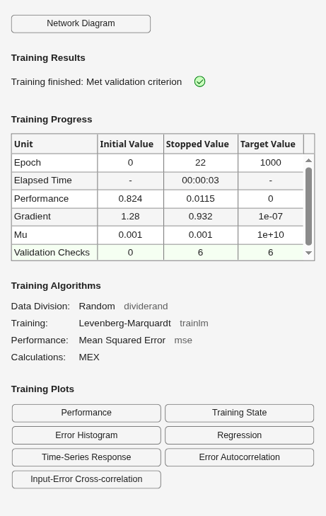
View the trained model.
view(model_narxnetCL2)
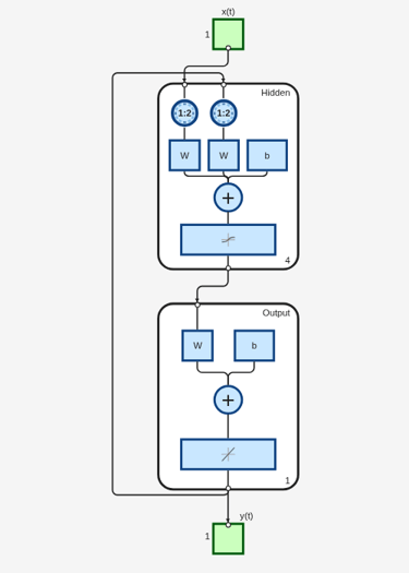
The model model_narxnet_CL2 is already in a closed-loop configuration. So there is no need to call the closeloop (Deep Learning Toolbox) command on it. Simulate the model output using the sim (Deep Learning Toolbox) command.
Ys2 = sim(model_narxnetCL2, XPredict, Xi2, Ai2);
Ys2 = cell2mat(Ys2)';
plot([y_measured,Ys1,Ys2])
legend("Measured","model_narxnetCL1","model_narxnetCL2",Interpreter="none")
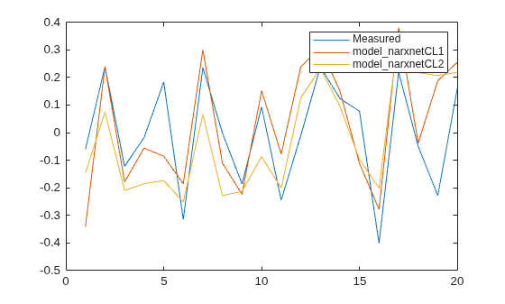
Measure the performance using goodnessOfFit with normalized root mean-squared error (NRMSE) metric.
err1 = goodnessOfFit(y_measured,Ys1,"nrmse")err1 = 0.7679
err2 = goodnessOfFit(y_measured,Ys2,"nrmse")err2 = 0.9685
nlarx Approach
Prepare data by converting the data used earlier into double vectors.
% training data
XTrain = cell2mat(XTrain)';
TTrain = cell2mat(TTrain)';
% validation data
XPredict = cell2mat(XPredict)';
YPredict = cell2mat(YPredict)';
Prepare model orders.
na = 2;
nb = 2;
nk = 1;
Order = [na nb nk];
Create a network function that is similar to the one used by the narxnet (Deep Learning Toolbox) models above using idNeuralNetwork. That is, create a network with one hidden tanh layer with 10 units. You can create the network by using the modern dlnetwork (Deep Learning Toolbox) object or the RegressionNeuralNetwork (Statistics and Machine Learning Toolbox) regression model.
netfcn = idNeuralNetwork(numUnits,"tanh",NetworkType="RegressionNeuralNetwork");
The neural network function netfcn employs a parallel connection of a linear map with a network. This is useful for semi-physical modeling, where you have the option to initialize the linear piece using an existing, possibly physics-based, transfer function. However, for this example, turn off the use of the linear map so that the structure of netfcn is equivalent to the one used by narxnet models.
netfcn.LinearFcn.Use = false;
Identify an nlarx model in open-loop. Use the LM training method.
Method = "lm";
opt = nlarxOptions(Focus="prediction",SearchMethod=Method);
model_nlarxOL = nlarx(XTrain,TTrain,Order,netfcn,opt)
model_nlarxOL =
Nonlinear ARX model with 1 output and 1 input
  Inputs: u1
  Outputs: y1

Regressors:
  Linear regressors in variables y1, u1
  List of all regressors

Output function: Regression neural network
Sample time: 1 seconds

Status:
Estimated using NLARX on time domain data "XTrain".
Fit to estimation data: 44.96% (prediction focus)
FPE: 0.0262, MSE: 0.0143

Model Properties
Train a model in closed-loop (this takes longer to train).
opt = nlarxOptions(Focus="simulation",SearchMethod=Method);
model_nlarxCL = nlarx(XTrain,TTrain,Order,netfcn,opt)
model_nlarxCL = Nonlinear ARX model with 1 output and 1 input Inputs: u1 Outputs: y1 Regressors: Linear regressors in variables y1, u1 List of all regressors Output function: Regression neural network Sample time: 1 seconds Status: Estimated using NLARX on time domain data "XTrain". Fit to estimation data: 39.74% (simulation focus) FPE: 0.03972, MSE: 0.01715 Model Properties
model_nlarxOL and model_nlarxCL are structurally similar and you can use either one for open-loop or closed-loop evaluation.
Perform open-loop evaluation using the predict command. In the system identification terminology, this exercise is called one-step-ahead prediction.
Horizon = 1; % prediction horizon
[yp1,ic1] = predict(XPredict,YPredict,model_nlarxOL,Horizon);
[yp2,ic2] = predict(XPredict,YPredict,model_nlarxCL,Horizon);
plot([y_measured,yp1,yp2])
legend("Measured","model_nlarxOL","model_nlarxCL",Interpreter="none")
title("One-step-ahead (open-loop) Prediction")
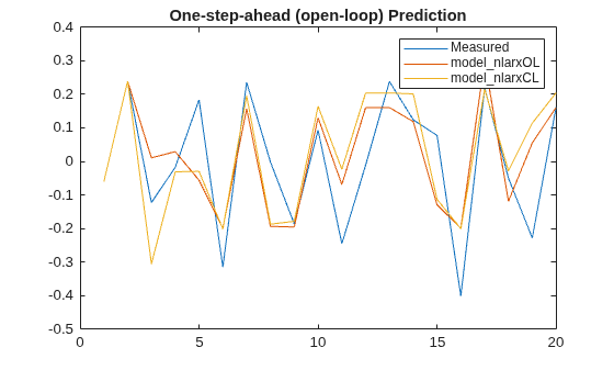
Measure the performance using goodnessOfFit with normalized root mean-squared error (NRMSE) metric.
err1 = goodnessOfFit(y_measured,yp1,"nrmse")err1 = 0.8896
err2 = goodnessOfFit(y_measured,yp2,"nrmse")err2 = 0.8474
Perform closed-loop evaluation using the sim command. In the system identification terminology, this exercise is called simulation or infinite-step-ahead prediction. You do not require the measured output (YPredict) for simulation.
ys1 = sim(model_nlarxOL,XPredict,simOptions(InitialCondition=ic1));
ys2 = sim(model_nlarxCL,XPredict,simOptions(InitialCondition=ic2));
plot([y_measured,ys1,ys2])
legend("Measured","model_nlarxOL","model_nlarxCL",Interpreter="none")
title("Closed-loop Prediction (Simulation)")
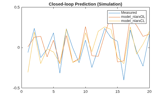
Measure the performance using goodnessOfFit with normalized root mean-squared error (NRMSE) metric.
err1 = goodnessOfFit(y_measured,ys1,"nrmse")err1 = 0.9848
err2 = goodnessOfFit(y_measured,ys2,"nrmse")err2 = 0.7975
See Also
train (Deep Learning Toolbox) | preparets (Deep Learning Toolbox) | closeloop (Deep Learning Toolbox) | narxnet (Deep Learning Toolbox) | idNeuralNetwork | idnlarx | nlarx | nlarxOptions | predict | iddata | linearRegressor | polynomialRegressor | getreg | periodicRegressor

