Neural State-Space Model of Simple Pendulum System
This example shows how to design and train a deep neural network that approximates a nonlinear state-space system in continuous time.
Neural State-Space Model
A state-space model is a representation of a dynamic system that uses a state equation and an output equation.
State equation:
Output equation:
Here, , , and are vectors representing the plant state, input, and measured output, respectively.
The state equation is a set of first-order ordinary differential equations (ODEs) or difference equations, which are often derived from first principles (white-box modeling). In practice, however, finding simple analytical equations that accurately describe your system is often hard because, for example, the system is complicated or some domain knowledge of its internal workings is missing or unobtainable.
In these cases, data-driven modeling (grey-box or black-box modeling) can be a useful alternative. One such data-driven approach is neural state-space modeling, which represents both the state and output equations of the nonlinear system by networks, as shown in this figure.

For example, for a continuous-time nonlinear system, you can use a multi-layer perceptron (MLP) network to approximate the state equation. The network inputs are and , the plant state and input vectors, and the network output is , the vector of plant state derivatives.
Similarly, when a nontrivial (that is) output equation exists, you can use another MLP network is to approximate it. For this network, the inputs are again and , while the network output is, the measured plant output.
Simple Pendulum
In this example, you create a neural state-space model of a simple forced pendulum. The pendulum has two states (angle and angular velocity ), one input (torque ), and two outputs (point mass horizontal position , point mass vertical position ).

To successfully identify the neural state-space model, the following prerequisites must be satisfied:
The state variables that you select must sufficiently describe the system behavior (for example, the current value of the state variables is all it is needed to predict future states, given the system equations). For physical plants, you can use domain knowledge to determine what plant variables are included in the state vector for the specific dynamics you want to model. If the desired set of states is not measurable, you have to choose an alternative set of states that can equivalently describe the system dynamic behavior. For example, if angle and angular velocity are not measurable in the simple pendulum problem, choose point mass position and its velocity as the state vector because it can sufficiently describe the pendulum behavior as long as they are measurable.
The states, inputs, and outputs (when) must be measurable, as the training data consists of state, input, and output trajectories collected during experiments.
For this example, you can assume that the states are sufficient to describe the system and that they and the outputs are measurable.
Design of Experiments
Design of Experiments (DoE) is a critical step in any data-driven modeling applications because in general, the quality of the model can only be as good as the quality of the data that you use to identify it. When you collect data for neural state-space modeling, make sure that the state trajectories cover the state space as much as possible under the operating conditions in design.
For this example, 101 experiments were conducted against a simulated plant (the ground-truth plant), each starting at different initial angle and angular velocity . Experiments lasted 1 second and state trajectories were logged every 0.1 seconds. During each experiment, the plant input (torque) was randomly changed within the bounds .
Load the data, which consists of two cell arrays of timetables: the state trajectories Y and the input trajectories U. Set N, the number of training experiments, to one less than the total number of experiments (that is, 100). Reserve the final experiment for validation.
load pendulumdata;
N = length(Y) - 1;
In practice, you often have restrictions on how many experiments can be carried out and how long an experiment can last due to operational, safety, and economic reasons. In this example, you can alternatively conduct 10 experiments that each lasts 10 seconds. You can divide each experiment into 10 segments, which is effectively equivalent to the original experiment, as long as the 10 state trajectories also cover enough state space.
Design Neural State Space Model
Define a neural state-space model with two states and one input. In the neural state-space model, since states are always included as the first outputs of the model, include four outputs. The first two outputs are states (angle and angular velocity) and the last two outputs are point mass horizontal and vertical positions.
sys = idNeuralStateSpace(2,NumInputs=1,NumOutput=4);
The state and output networks are initialized randomly. For reproducibility, fix the random seed generator.
rng(0);
Now, customize the state and output networks by creating MLP networks for each. Note that when the output equation is not trivial, as in this example, the OutputNetwork property contains a vector of two neural networks, the first one representing and the second one representing the output equation. Therefore, when you customize the network for the output equation, update OutputNetwork(2).
% State network
sys.StateNetwork = createMLPNetwork(sys,'state', ...
   LayerSizes=[128 128], ...
   Activations="tanh", ...
   WeightsInitializer="glorot", ...
   BiasInitializer="zeros");

% Output network
sys.OutputNetwork(2) = createMLPNetwork(sys,'output', ...
   LayerSizes=[128 128], ...
   Activations="tanh", ...
   WeightsInitializer="glorot", ...
   BiasInitializer="zeros");
Train Neural State Space Model
Create a training options object with the solver set to 'adam'. Set the maximum number of epochs to 200 and the learning rate to 0.005.
options = nssTrainingOptions('adam');
options.MaxEpochs = 200;
options.LearnRate = 0.005;
The model has more parameters than data samples, which causes a warning. Suppress this warning before calling nlssest.
Warn = warning('off','Ident:estimation:NparGTNsamp');
WarnReset = onCleanup(@()warning(Warn));
To train the neural state-space model, use nlssest. To use the last experiment in the data set for the validation plot, set the UseLastExperimentForValidation argument to true in the command.
sys = nlssest(U,Y,sys,options,UseLastExperimentForValidation=true);


Generating estimation report...done.
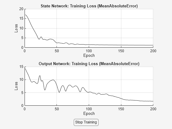
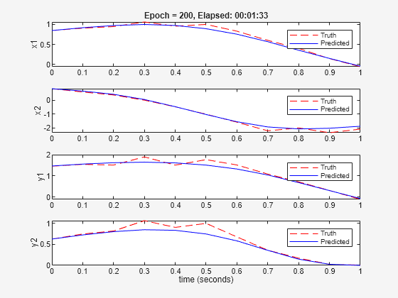
During training, two plots are displayed for examination. The first plot displays loss values against completed epochs for both networks. The second plot displays predicted state and output trajectories against the measured trajectories based on the validation data set.
Analyze Trained Neural State Space Model
A neural state-space model provides commands to facilitate analysis and use of a trained model. For example, you can use evaluate to compute state derivatives and outputs given state and input.
x0 = rand(2,1);
u0 = rand;
[dxdt,y] = evaluate(sys,x0,u0);
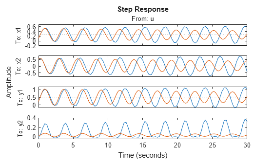
Use linearize to create a LTI state-space model at a specified operating point. Compare the step response of the linear model with that of the original one.
sysLinear = linearize(sys,x0,u0);
opt = RespConfig(InputOffset=u0,InitialState=x0);
step(sys,sysLinear,30,opt)

You can generate standalone MATLAB® functions for the state and output functions, and their Jacobians, from the neural state-space model. You can use these functions to simulate the neural state-space system and to generate C/C++ code for deployment purposes, for applications such as nonlinear state estimation and model predictive control.
generateMATLABFunction(sys,"myStateFcn","myOutputFcn");
Wait until the files are written and made accessible by the file system.
while ~exist("myStateFcn","file")
    pause(1);
end
while ~exist("myOutputFcn","file")
    pause(1);
end
Call the state and output functions to display the state derivative and the output at the operating point.
dxdt1 = myStateFcn(x0,u0)
dxdt1 = 2×1

    0.4491
   -2.7142
y1 = myOutputFcn(x0,u0)
y1 = 2×1

    1.1843
    0.4245
Calling these functions produces the same answer as calling evaluate on the neural state-space object itself.
error = norm([dxdt;y(3:4)]-[dxdt1;y1])
error =
0
You can also use other System Identification Toolbox™ commands such as sim, predict, and compare on the neural state-space model.
See Also
Objects
Functions
createMLPNetwork|nssTrainingOptions|nlssest|generateMATLABFunction|idNeuralStateSpace/evaluate|idNeuralStateSpace/linearize|sim