Automate Pixel Labeling of Hyperspectral Images Using Image Labeler
This example shows how to load hyperspectral images into the Image Labeler (Computer Vision Toolbox) and automatically label pixels.
In this example, you load hyperspectral image data into the Image Labeler and assign pixel labels using an automation algorithm. The automation algorithm matches the spectral signature of each pixel with the spectral signatures of labeled pixels or spectral signatures from the ECOSTRESS library and annotates every pixel automatically using the spectral angle mapper (SAM) classification algorithm.
This example requires the Hyperspectral Imaging Library for Image Processing Toolbox™. You can install the Hyperspectral Imaging Library for Image Processing Toolbox from Add-On Explorer. For more information about installing add-ons, see Get and Manage Add-Ons. The Hyperspectral Imaging Library for Image Processing Toolbox requires desktop MATLAB®, as MATLAB® Online™ and MATLAB® Mobile™ do not support the library.
Import Hyperspectral Image into Image Labeler
To make the multi-channel hyperspectral images suitable for importing into the Image Labeler, load the hyperspectral images as an image datastore using the custom read function readColorizedHyperspectralImage, defined at the end of this example. The custom read function returns a 3-channel image for the Image Labeler to display.
file = "jasperRidge2_R198.img";
imds = imageDatastore(file,ReadFcn=@readColorizedHyperspectralImage,FileExtensions=".img");
You can use the Hyperspectral Viewer app to explore colorization methods that help accentuate regions of interest within the data. For the Jasper Ridge data, the colorize function with Method specified as "falsecolored" returns a false-colored image using bands 145, 99, and 19.
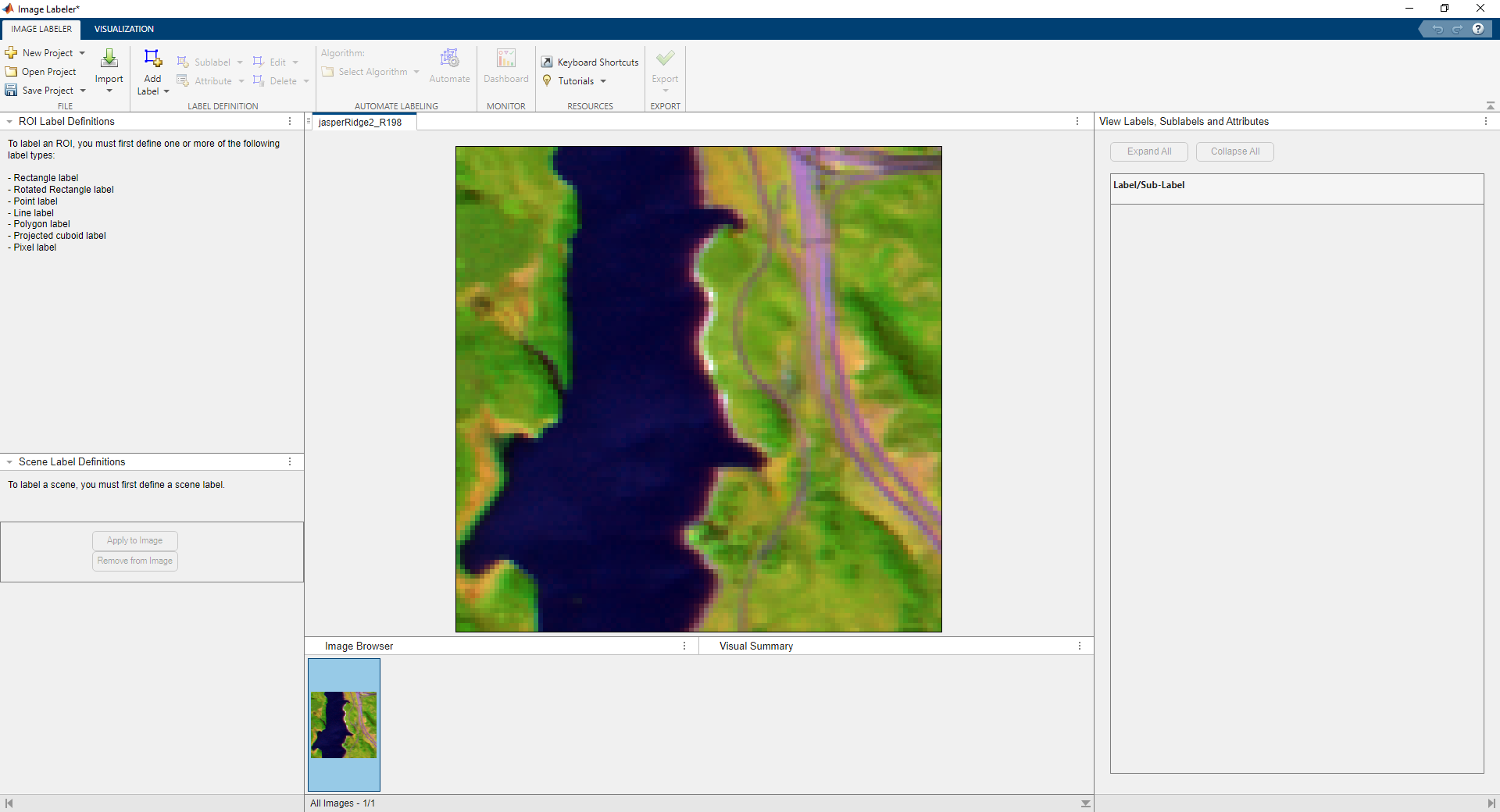
Open the Image Labeler app. First, select the Apps tab on the MATLAB toolstrip. Then, in the Image Processing and Computer Vision section, select Image Labeler. Alternatively, you can open the Image Labeler app programmatically by entering this command at the MATLAB Command Prompt.
imageLabeler
On the Image Labeler Start Page, select New Individual Project.

Perform these steps to import the image datastore imds into the Image Labeler.
On the Image Labeler tab of the app toolstrip, select Import, and then select From Workspace.
Use the dialog box to select the image datastore
imds.
Define Pixel Labels
The Jasper Ridge hyperspectral image contains spectral signatures that help classify the types of material in the image. The materials known to be present in the image are sea water, vegetation, soil (utisol and mollisol), and concrete. Perform these steps for each class to define pixel labels for the five classes.
On the Image Labeler tab, select Add Label and then select Pixel.
In the dialog box, enter
SeaWateras the name for the pixel label and select OK.Repeat this process for the remaining material types,
Tree,Utisol,Mollisol, andConcrete.
Alternatively, you can use the labelDefinitionCreator (Computer Vision Toolbox) function to programmatically create pixel label definitions for the five classes.
classes = ["SeaWater","Tree","Utisol","Mollisol","Concrete"];
ldc = labelDefinitionCreator;
for i = 1:numel(classes)
    addLabel(ldc,classes(i),labelType.PixelLabel)
end
labelDefinitions = create(ldc)
labelDefinitions=5×6 table
        Name           Type       LabelColor    PixelLabelID     Group      Description
    ____________    __________    __________    ____________    ________    ___________

    {'SeaWater'}    PixelLabel    {0×0 char}       {[1]}        {'None'}       {' '}
    {'Tree'    }    PixelLabel    {0×0 char}       {[2]}        {'None'}       {' '}
    {'Utisol'  }    PixelLabel    {0×0 char}       {[3]}        {'None'}       {' '}
    {'Mollisol'}    PixelLabel    {0×0 char}       {[4]}        {'None'}       {' '}
    {'Concrete'}    PixelLabel    {0×0 char}       {[5]}        {'None'}       {' '}
Save the label definition table to a MAT file.
save JasperRidgeLabelDefinitions.mat labelDefinitions
Perform these steps to import the label definitions into the Image Labeler app.
On the Image Labeler tab, select Import, and then select Label Definitions.
In the dialog box, select the file
JasperRidgeLabelDefinitions.mat.
Label Pixels in Image Labeler
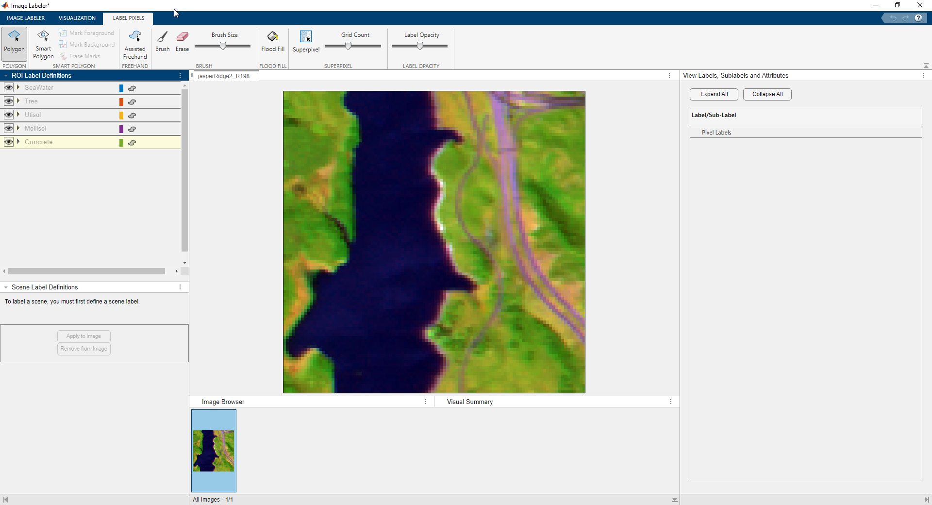
Because you can visually distinguish the SeaWater in the image, label seed pixels for this class in the Image Labeler app, and use the mean spectral signature of the labeled seed pixels to automatically label the rest of the pixels of this class.
Perform these steps to label seed pixels for the SeaWater class.
In the ROI Label Definitions pane, select the
SeaWaterclass.On the app toolstrip, in the Label Pixels tab, select Brush.
Label water pixels in the image using the brush.
Save the current labeling project using the Save Project option on the Image Labeler tab.

Define Automation Algorithm
Automation algorithms implement an API that enables the Image Labeler app to call user-defined algorithms for labeling. For hyperspectral images, you can define automation algorithms based on spectral matching, object detection networks, semantic segmentation networks, and so on, for pixel labeling. This example uses an automation algorithm based on spectral matching. For more information on writing an automation algorithm, see Create Automation Algorithm for Labeling (Computer Vision Toolbox).
The ECOSTRESS spectral library consists of over 3400 spectral signatures for both natural and manmade surface materials. You can automatically label the pixels by matching the spectra of each pixel to either the mean spectral signature of your labeled seed pixels of a class or to the spectral signatures in the library. Use the spectral angle mapping (SAM) technique in the automation algorithm class SpectralAngleMapperAutomationAlgorithm for labeling the pixels. The automation algorithm class SpectralAngleMapperAutomationAlgorithm is attached to this example as a supporting file.
Create a +vision/+labeler/ folder within the current working folder. Copy the automation algorithm class file SpectralAngleMapperAutomationAlgorithm.m to the folder +vision/+labeler.
exampleFolder = pwd;
automationFolder = fullfile("+vision","+labeler");
mkdir(exampleFolder,automationFolder)
copyfile("SpectralAngleMapperAutomationAlgorithm.m",automationFolder)
These are the key components of the automation algorithm class.
The
SpectralAngleMapperAutomationAlgorithmconstructorThe
settingsDialogmethodThe
runmethod
The constructor uses the readEcostressSig function to load all the ECOSTRESS spectral signatures provided within the Image Processing Toolbox Hyperspectral Imaging Library. You can modify the constructor to add more spectral signatures from the ECOSTRESS library.
function this = SpectralAngleMapperAutomationAlgorithm()

    % List the ECOSTRESS files containing material signatures
    % present in the data to be labeled. Modify this list as
    % needed based on the data to be labeled.
    filenames = [
        "manmade.concrete.pavingconcrete.solid.all.0092uuu_cnc.jhu.becknic.spectrum.txt"
        "manmade.road.tar.solid.all.0099uuutar.jhu.becknic.spectrum.txt"
        "manmade.roofingmaterial.metal.solid.all.0384uuualm.jhu.becknic.spectrum.txt"
        "manmade.roofingmaterial.metal.solid.all.0692uuucop.jhu.becknic.spectrum.txt"
        "soil.mollisol.cryoboroll.none.all.85p4663.jhu.becknic.spectrum.txt"
        "soil.utisol.hapludult.none.all.87p707.jhu.becknic.spectrum.txt"
        "vegetation.grass.avena.fatua.vswir.vh353.ucsb.asd.spectrum.txt"
        "vegetation.tree.abies.concolor.tir.vh063.ucsb.nicolet.spectrum.txt"
        "vegetation.tree.bambusa.tuldoides.tir.jpl216.jpl.nicolet.spectrum.txt"
        "vegetation.tree.eucalyptus.maculata.vswir.jpl087.jpl.asd.spectrum.txt"
        "vegetation.tree.pinus.ponderosa.tir.vh254.ucsb.nicolet.spectrum.txt"
        "vegetation.tree.tsuga.canadensis.vswir.tsca-1-47.ucsb.asd.spectrum.txt"
        "water.ice.none.solid.all.ice_dat_.jhu.becknic.spectrum.txt"
        "water.seawater.none.liquid.tir.seafoam.jhu.becknic.spectrum.txt"
        "water.tapwater.none.liquid.all.tapwater.jhu.becknic.spectrum.txt"
        ];

    % Load the ECOSTRESS signatures.
    this.EcostressSignatures = readEcostressSig(filenames);

end
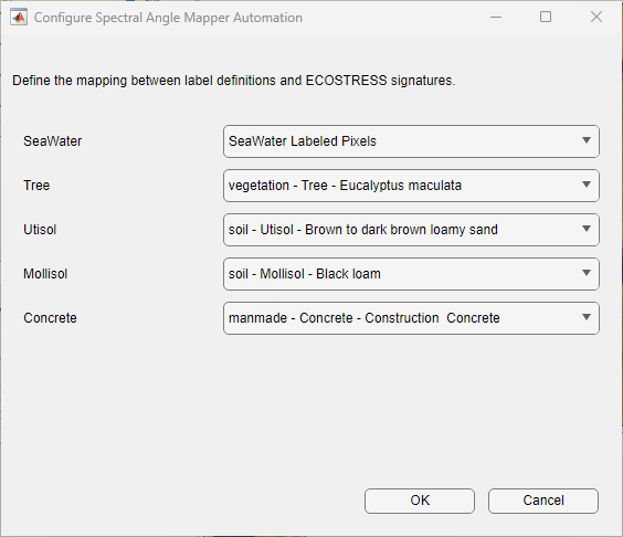
The settingsDialog method launches a custom dialog box that enables you to map label definitions to spectral signatures. The settingsDialog method uses the SAMSettings class, which has been generated, using the App Designer, to create the custom dialog design and modified to support a dynamic number of spectral signatures. The SAMSettings class is attached to this example as a supporting file. Ensure this file remains in the current working folder. Use the dialog box to map the label definitions to spectral signatures before running the automation algorithm.
The run method of the automation algorithm loads the hyperspectral image, runs the spectral matching algorithm, and returns a categorical array containing the pixel labels. You can use a similar approach to implement other automation algorithms that require processing all the bands within the hyperspectral data.
function C = run(this, ~)

    % Load the hyperspectral image being processed using the
    % CurrentIndex property.
    src = this.GroundTruth.DataSource;
    filename = src.Source.Files{this.CurrentIndex};
    hcube = hypercube(filename);
    datacube = gather(hcube);
    [M,N,C] = size(datacube);
    flatDataCube = reshape(datacube,[],C)';

    % Match hypercube spectra with selected signatures
    ecoSigIdx = this.SelectedSigIdx(this.SelectedSigIdx<=length(this.EcostressSignatures));
    ecoSigSpectra = {this.EcostressSignatures(ecoSigIdx).Reflectance};
    ecoSigWavelength = {this.EcostressSignatures(ecoSigIdx).Wavelength};
    labeledSigIdx = this.SelectedSigIdx(this.SelectedSigIdx>length(this.EcostressSignatures));
    labeledSigIdx = sort(labeledSigIdx) - length(this.EcostressSignatures);
    labeledSigSpectra = cell(1,1);
    labeledSigWavelength = cell(1,1);
    tempFile = string(this.GroundTruth.LabelData.PixelLabelData(1));
    labelData = imread(tempFile);
    for i = labeledSigIdx
        labelLoc = labelData==i;
        labelLoc = reshape(labelLoc,[],1)';
        labeledSigSpectra(i) = {mean(flatDataCube(:,labelLoc),2)};
        labeledSigWavelength(i) = {hcube.Wavelength};
    end
    selectedSigSpectra = [ecoSigSpectra labeledSigSpectra];
    selectedSigWavelength = [ecoSigWavelength labeledSigWavelength];
    scores = zeros(M,N,numel(selectedSigSpectra));
    for i = 1:numel(selectedSigSpectra)
        [refSpectra,~,wIndex] = resampleSignature(selectedSigSpectra{i},hcube.Wavelength,selectedSigWavelength{i});
        scores(:,:,i) = sam(datacube(:,:,wIndex(1):wIndex(2)),refSpectra);
    end

    % Classify the spectral signatures by finding the minimum score.
    [~,L] = min(scores,[],3);

    % Determine the pixel label classes.
    pxLabels = this.GroundTruth.LabelDefinitions.Type == labelType.PixelLabel;
    def = this.GroundTruth.LabelDefinitions(pxLabels,:);
    classes = def.Name;

    % Return a categorical image
    C = categorical(L,1:numel(this.SelectedSigIdx),classes);

end
Import Automation Algorithm
Import the automation algorithm into the Image Labeler app by performing these steps.
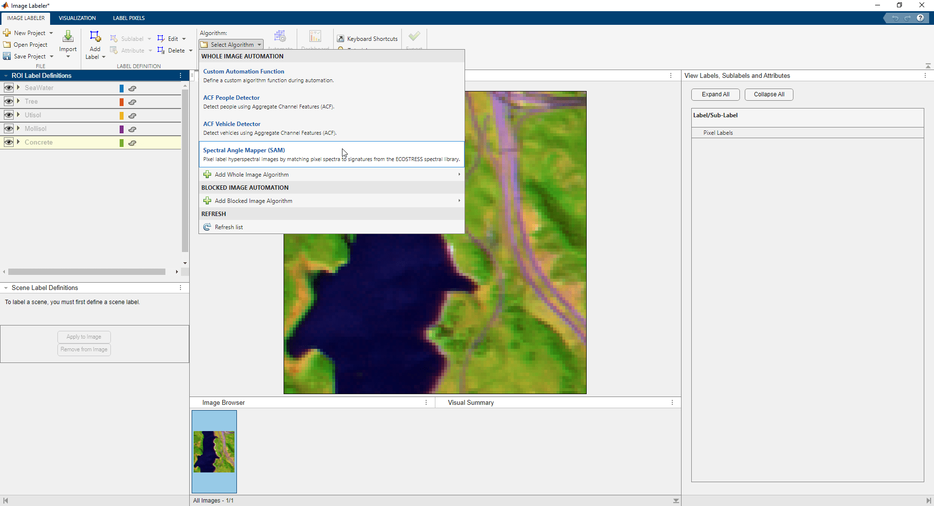
On the Image Labeler tab, select Select Algorithm.
Select Add Whole Image Algorithm, and then select Import Algorithm.
Navigate to the
+vision/+labelerfolder in the current working folder and chooseSpectralAngleMapperAutomationAlgorithm.mfrom the file selection dialog box.
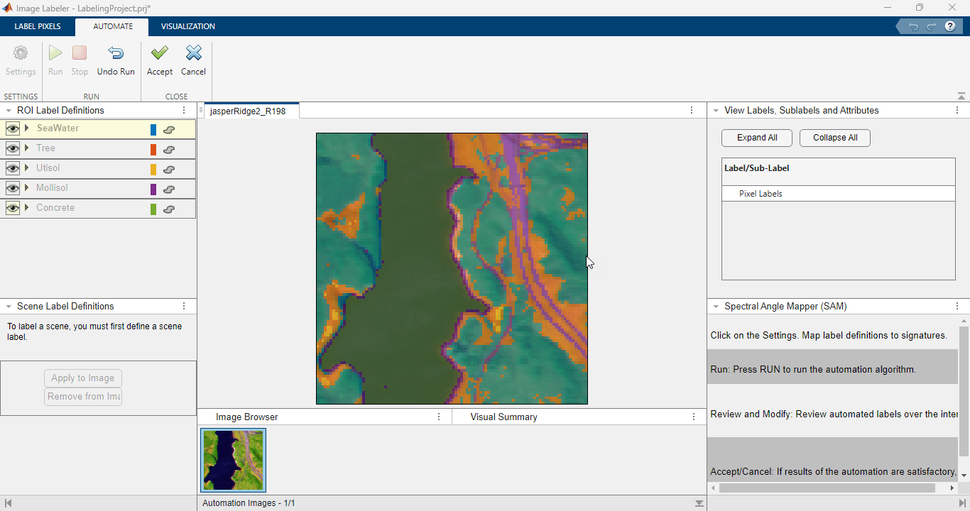
Run Automation Algorithm
Perform these steps to configure the automation algorithm.
On the Image Labeler tab, select Automate. This creates the Automate tab.
On the Automate tab, select Settings. This opens the settings dialog created using the
settingsDialogmethod in the automation algorithm. Use the settings dialog to map label definitions to the corresponding spectral signatures. You can either select spectral signatures of labeled seed pixels or spectral signatures from the ECOSTRESS library for each class.

Perform these steps to run the configured automation algorithm.
On the Automate tab, select Run.
Review the automation results. Use the tools in the Label Pixels tab to correct any automation errors.
If the labels are satisfactory then, on the Automate tab, select Accept, in the Automate tab.
Export Ground Truth Labels
Perform these steps to export the label data for the hyperspectral image.
Save the current labeling project using the Save Project option on the Image Labeler tab. After selecting Save Project, select Save. Specify a name for the labeling project and click Save.
On the Image Labeler tab, select Export, and then select To Workspace.
Specify the location and name of the workspace variable to which you want to save the ground truth label data.
You can use the exported ground truth in downstream tasks, such as for training a deep learning network or verifying the results of hyperspectral image processing algorithms.
Supporting Functions
function colorizedImg = readColorizedHyperspectralImage(file)
    % Colorize the hyperspectral image using false coloring to accentuate regions of interest within the data.
    hcube = imhypercube(file);
    colorizedImg = colorize(hcube,Method="falsecolored");
end
References
[1] Kruse, F.A., A.B. Lefkoff, J.W. Boardman, K.B. Heidebrecht, A.T. Shapiro, P.J. Barloon, and A.F.H. Goetz. “The Spectral Image Processing System (SIPS)—Interactive Visualization and Analysis of Imaging Spectrometer Data.” Remote Sensing of Environment 44, no. 2–3 (May 1993): 145–63. https://doi.org/10.1016/0034-4257(93)90013-N.
[2] ECOSTRESS Spectral Library: https://speclib.jpl.nasa.gov
[3] Meerdink, Susan K., Simon J. Hook, Dar A. Roberts, and Elsa A. Abbott. “The ECOSTRESS Spectral Library Version 1.0.” Remote Sensing of Environment 230 (September 2019): 111196. https://doi.org/10.1016/j.rse.2019.05.015.
[4] Baldridge, A.M., S.J. Hook, C.I. Grove, and G. Rivera. “The ASTER Spectral Library Version 2.0.” Remote Sensing of Environment 113, no. 4 (April 2009): 711–15. https://doi.org/10.1016/j.rse.2008.11.007.
See Also
Image Labeler (Computer Vision Toolbox)