Aerial Lidar SLAM Using FPFH Descriptors

This example uses:

This example demonstrates how to implement the simultaneous localization and mapping (SLAM) algorithm for aerial mapping using 3-D features. The goal of this example is to estimate the trajectory of a robot and create a point cloud map of its environment.

The SLAM algorithm in this example estimates a trajectory by finding a coarse alignment between downsampled accepted scans, using fast point feature histogram (FPFH) descriptors extracted at each point, then applies the iterative closest point (ICP) algorithm to fine-tune the alignment. 3-D pose graph optimization, from Navigation Toolbox™, reduces the drift in the estimated trajectory.

Create and Visualize Data

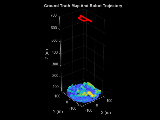
Create synthetic lidar scans from a patch of aerial data, downloaded from the OpenTopography website [1]. Load a MAT-file containing a sequence of waypoints over aerial data that defines the trajectory of a robot. Compute lidar scans from the data at each waypoint using the helperCreateDataset function. The function outputs the lidar scans computed at each waypoint as an array of pointCloud objects, original map covered by robot and ground truth waypoints.

datafile = 'aerialMap.tar.gz';
wayPointsfile = 'gTruthWayPoints.mat';

% Generate a lidar scan at each waypoint using the helper function
[pClouds,orgMap,gTruthWayPts] = helperCreateDataset(datafile,wayPointsfile);

Visualize the ground truth waypoints on the original map covered by the robot.

% Create a figure window to visualize the ground truth map and waypoints
hFigGT = figure;
axGT = axes(Parent=hFigGT,Color='black');

% Visualize the ground truth waypoints
pcshow(gTruthWayPts,'red',MarkerSize=150,Parent=axGT)
hold on

% Visualize the original map covered by the robot
pcshow(orgMap,MarkerSize=10,Parent=axGT)
hold off

% Customize the axis labels
axis on
xlabel(axGT,'X (m)')
ylabel(axGT,'Y (m)')
zlabel(axGT,'Z (m)')
title(axGT,'Ground Truth Map And Robot Trajectory')

Figure contains an axes object. The axes object with title Ground Truth Map And Robot Trajectory, xlabel X (m), ylabel Y (m) contains 2 objects of type scatter.

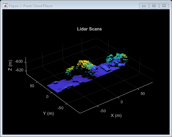
Visualize the extracted lidar scans using the pcplayer object.

% Specify limits for the player
xlimits = [-90 90];
ylimits = [-90 90];
zlimits = [-625 -587];

% Create a pcplayer object to visualize the lidar scans
lidarPlayer = pcplayer(xlimits,ylimits,zlimits);

% Customize the pcplayer axis labels
xlabel(lidarPlayer.Axes,'X (m)')
ylabel(lidarPlayer.Axes,'Y (m)')
zlabel(lidarPlayer.Axes,'Z (m)')
title(lidarPlayer.Axes,'Lidar Scans')

% Loop over and visualize the data
for l = 1:length(pClouds)

    % Extract the lidar scan
    ptCloud = pClouds(l);

    % Update the lidar display
    view(lidarPlayer,ptCloud)
    pause(0.05)
end

Figure Point Cloud Player contains an axes object. The axes object with title Lidar Scans, xlabel X (m), ylabel Y (m) contains an object of type scatter.

Set Up Tunable Parameters

Specify the parameters for trajectory and loop closure estimation. Tune these parameters for your specific robot and environment.

Parameters for Point Cloud Registration

Specify the number of lidar scans to skip between each scan accepted for registration. Since successive scans have high overlap, skipping a few frames can improve algorithm speed without compromising accuracy.

skipFrames = 3;

Downsampling lidar scans can improve algorithm speed. The box grid filter downsamples the point cloud by averaging all points within each cell to a single point. Specify the size for individual cells of a box grid filter, in meters.

gridStep = 1.5; % in meters

FPFH descriptors are extracted for each valid point in the downsampled point cloud. Specify the neighborhood size for the k-nearest neighbor (KNN) search method used to compute the descriptors.

neighbors = 60;

Set the threshold and ratio for matching the FPFH descriptors, used to identify point correspondences.

matchThreshold = 0.1;
matchRatio = 0.97;

Set the maximum distance and number of trails for relative pose estimation between successive scans.

maxDistance = 1;
maxNumTrails = 3000;

Specify plane-to-plane minimization metric and inlier distance threshold between the points for registration.

metric = "planeToPlane";
inlierDistance = 3;

Specify the size of each cell of a box grid filter, used to create maps by aligning lidar scans.

alignGridStep = 1.2;

Parameters for Loop Closure Estimation

Specify the radius around the current robot location to search for loop closure candidates.

loopClosureSearchRadius = 7.9;

The loop closure algorithm is based on 3-D submap creation and matching. A submap consists of a specified number of accepted scans nScansPerSubmap. The loop closure algorithm also disregards a specified number of the most recent scans subMapThresh, while searching for loop candidates. Specify the root mean squared error (RMSE) threshold loopClosureThreshold, for accepting a submap as a match. A lower score can indicate a better match, but scores vary based on sensor data and preprocessing.

nScansPerSubmap = 3;
subMapThresh = 15;
loopClosureThreshold = 0.6;

Specify the maximum acceptable root mean squared error (RMSE) for the estimation of relative pose between loop candidates rmseThreshold. Choosing a lower value can result in more accurate loop closure edges, which has a high impact on pose graph optimization, but scores vary based on sensor data and preprocessing.

rmseThreshold = 0.6;

Initialize Variables

Create a pose graph, using a poseGraph3D (Navigation Toolbox) object, to store estimated relative poses between accepted lidar scans.

pGraph = poseGraph3D;

% Default serialized upper-right triangle of a 6-by-6 Information Matrix
infoMat = [1 0 0 0 0 0 1 0 0 0 0 1 0 0 0 1 0 0 1 0 1];

Preallocate and initialize the variables required for computation.

% Allocate memory to store submaps
subMaps = cell(floor(length(pClouds)/(skipFrames*nScansPerSubmap)),1);

% Allocate memory to store each submap pose
subMapPoses = zeros(round(length(pClouds)/(skipFrames*nScansPerSubmap)),3);

% Initialize variables to store accepted scans and their transforms for
% submap creation
pcAccepted = pointCloud.empty(0);
tformAccepted = rigidtform3d.empty(0);

% Initialize variable to store relative poses from the feature-based approach
% without pose graph optimization
fpfhTform = rigidtform3d.empty(0);

% Counter to track the number of scans added
count = 1;

Create variables to visualize processed lidar scans and estimated trajectory.

% Set to 1 to visualize processed lidar scans during build process
viewPC = 0;

% Create a pcplayer object to view the lidar scans while
% processing them sequentially, if viewPC is enabled
if viewPC == 1
    pplayer = pcplayer(xlimits,ylimits,zlimits);

    % Customize player axis labels
    xlabel(pplayer.Axes,'X (m)')
    ylabel(pplayer.Axes,'Y (m)')
    zlabel(pplayer.Axes,'Z (m)')
    title(pplayer.Axes,'Processed Scans')
end

% Create a figure window to visualize the estimated trajectory
hFigTrajUpdate = figure;
axTrajUpdate = axes(Parent=hFigTrajUpdate,Color='black');
title(axTrajUpdate,'Sensor Pose Trajectory')

Trajectory Estimation and Refinement

The trajectory of the robot is a collection of its poses which consists of its location and orientation in 3-D space. Estimate a robot pose from a 3-D lidar scan instance using the 3-D lidar SLAM algorithm. Use these processes to perform 3-D SLAM estimation:

Point cloud downsampling
Point cloud registration
Submap creation
Loop closure querying
Pose graph optimization

Iteratively process the lidar scans to estimate the trajectory of the robot.

rng('default') % Set random seed to guarantee consistent results in pcmatchfeatures
for FrameIdx = 1:skipFrames:length(pClouds)

Point Cloud Downsampling

Point cloud downsampling can improve the speed of the point cloud registration algorithm. Downsampling should be tuned for your specific needs.

    % Downsample the current scan
    curScan = pcdownsample(pClouds(FrameIdx),gridAverage=gridStep);
    if viewPC == 1

        % Visualize down sampled point cloud
        view(pplayer,curScan)
    end

Point Cloud Registration

Point cloud registration estimates the relative pose between the current scan and a previous scan. The example uses these steps for registration:

Extracts FPFH descriptors from each scan using the extractFPFHFeatures function
Identifies point correspondences by comparing descriptors using the pcmatchfeatures function
Estimates the relative pose from point correspondences using the estgeotform3d function
Fine-tunes the relative pose using the pcregistericp function

    % Extract FPFH features
    curFeature = extractFPFHFeatures(curScan,NumNeighbors=neighbors);

    if FrameIdx == 1

        % Update the acceptance scan and its tform
        pcAccepted(count,1) = curScan;
        tformAccepted(count,1) = rigidtform3d;

        % Update the initial pose to the first waypoint of ground truth for
        % comparison
        fpfhTform(count,1) = rigidtform3d([0 0 0],gTruthWayPts(1,:));
    else

        % Identify correspondences by matching current scan to previous scan
        indexPairs = pcmatchfeatures(curFeature,prevFeature,curScan,prevScan, ...
            MatchThreshold=matchThreshold,RejectRatio=matchRatio);
        matchedPrevPts = select(prevScan,indexPairs(:,2));
        matchedCurPts = select(curScan,indexPairs(:,1));

        % Estimate relative pose between current scan and previous scan
        % using correspondences
        tform1 = estgeotform3d(matchedCurPts.Location, ...
            matchedPrevPts.Location,'rigid',MaxDistance=maxDistance, ...
            MaxNumTrials=maxNumTrails);

        % Perform ICP registration to fine-tune relative pose
        tform = pcregistericp(curScan,prevScan,InitialTransform=tform1, ...
            Metric=metric,InlierDistance=inlierDistance);

Convert the rigid transformation to an xyz-position and a quaternion orientation to add it to the pose graph.

        relPose = [tform2trvec(tform.A) tform2quat(tform.A)];

        % Add relative pose to pose graph
        addRelativePose(pGraph,relPose);

Store the accepted scans and their poses for submap creation.

        % Update counter and store accepted scans and their poses
        count = count + 1;
        pcAccepted(count,1) = curScan;
        accumPose = pGraph.nodes(height(pGraph.nodes));
        tformAccepted(count,1) = rigidtform3d((trvec2tform(accumPose(1:3)) * ...
            quat2tform(accumPose(4:7))));

        % Update estimated poses
        fpfhTform(count) = rigidtform3d(fpfhTform(count-1).A * tform.A);
    end

Submap Creation

Create submaps by aligning sequential, accepted scans with each other in groups of the specified size nScansPerSubmap, using the pcalign function. Using submaps can result in faster loop closure queries.

    currSubMapId = floor(count/nScansPerSubmap);
    if rem(count,nScansPerSubmap) == 0

        % Align an array of lidar scans to create a submap
        subMaps{currSubMapId} = pcalign(...
            pcAccepted((count - nScansPerSubmap + 1):count,1), ...
            tformAccepted((count - nScansPerSubmap + 1):count,1), ...
            alignGridStep);

        % Assign center scan pose as pose of submap
        subMapPoses(currSubMapId,:) = tformAccepted(count - ...
            floor(nScansPerSubmap/2),1).Translation;
    end

Loop Closure Query

Use a loop closure query to identify previously visited places. A loop closure query consists of finding a similarity between the current scan and previous submaps. If you find a similar scan, then the current scan is a loop closure candidate. Loop closure candidate estimation consists of these steps:

Estimate matches between previous submaps and the current scan using the helperEstimateLoopCandidates function. A submap is a match, if the RMSE between the current scan and submap is less than the specified value of loopClosureThreshold. The previous scans represented by all matching submaps are loop closure candidates.
Compute the relative pose between the current scan and the loop closure candidate using the ICP registration algorithm. The loop closure candidate with the lowest RMSE is the best probable match for the current scan.

A loop closure candidate is accepted as a valid loop closure only when the RMSE is lower than the specified threshold.

    if currSubMapId > subMapThresh
        mostRecentScanCenter = pGraph.nodes(height(pGraph.nodes));

        % Estimate possible loop closure candidates by matching current
        % scan with submaps
        [loopSubmapIds,~] = helperEstimateLoopCandidates(subMaps,curScan, ...
            subMapPoses,mostRecentScanCenter,currSubMapId,subMapThresh, ...
            loopClosureSearchRadius,loopClosureThreshold,metric,inlierDistance);

        if ~isempty(loopSubmapIds)
            rmseMin = inf;

            % Estimate the best match for the current scan from the matching submap ids
            for k = 1:length(loopSubmapIds)

                % Check every scan within the submap
                for kf = 1:nScansPerSubmap
                    probableLoopCandidate = ...
                        loopSubmapIds(k)*nScansPerSubmap - kf + 1;
                    [pose_Tform,~,rmse] = pcregistericp(curScan, ...
                        pcAccepted(probableLoopCandidate),Metric=metric, ...
                        InlierDistance=inlierDistance);

                    % Update the best loop closure candidate
                    if rmse < rmseMin
                        rmseMin = rmse;
                        matchingNode = probableLoopCandidate;
                        Pose = [tform2trvec(pose_Tform.A) ...
                            tform2quat(pose_Tform.A)];
                    end
                end
            end

            % Check if loop closure candidate is valid
            if rmseMin < rmseThreshold

                % Add relative pose of loop closure candidate to pose graph
                addRelativePose(pGraph,Pose,infoMat,matchingNode, ...
                    pGraph.NumNodes);
            end
        end
    end

    % Update previous point cloud and feature
    prevScan = curScan;
    prevFeature = curFeature;

    % Visualize the estimated trajectory from the accepted scan.
    show(pGraph,IDs='off',Parent=axTrajUpdate);
    drawnow
end

Figure contains an axes object. The axes object with xlabel X, ylabel Y contains 2 objects of type line. One or more of the lines displays its values using only markers

Figure contains an axes object. The axes object with xlabel X, ylabel Y contains 3 objects of type line. One or more of the lines displays its values using only markers

Pose Graph Optimization

Reduce the drift in the estimated trajectory by using the optimizePoseGraph (Navigation Toolbox) function. In general, the pose of the first node in the pose graph represents the origin. To compare the estimated trajectory with the ground truth waypoints, specify the first ground truth waypoint as the pose of the first node.

pGraph = optimizePoseGraph(pGraph,FirstNodePose=[gTruthWayPts(1,:) 1 0 0 0]);

Visualize Trajectory Comparisons

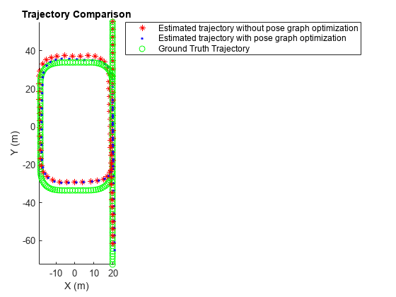
Visualize the estimated trajectory using the features without pose graph optimization, the features with pose graph optimization, and the ground truth data.

% Get estimated trajectory from pose graph
pGraphTraj = pGraph.nodes;

% Get estimated trajectory from feature-based registration without pose
% graph optimization
fpfhEstimatedTraj = zeros(count,3);
for i = 1:count
    fpfhEstimatedTraj(i,:) = fpfhTform(i).Translation;
end

% Create a figure window to visualize the ground truth and estimated
% trajectories
hFigTraj = figure;
axTraj = axes(Parent=hFigTraj,Color='black');
plot3(fpfhEstimatedTraj(:,1),fpfhEstimatedTraj(:,2),fpfhEstimatedTraj(:,3), ...
    'r*',Parent=axTraj)
hold on
plot3(pGraphTraj(:,1),pGraphTraj(:,2),pGraphTraj(:,3),'b.',Parent=axTraj)
plot3(gTruthWayPts(:,1),gTruthWayPts(:,2),gTruthWayPts(:,3),'go',Parent=axTraj)
hold off
axis equal
view(axTraj,2)
xlabel(axTraj,'X (m)')
ylabel(axTraj,'Y (m)')
zlabel(axTraj,'Z (m)')
title(axTraj,'Trajectory Comparison')
legend(axTraj,'Estimated trajectory without pose graph optimization', ...
    'Estimated trajectory with pose graph optimization', ...
    'Ground Truth Trajectory','Location','bestoutside')

Figure contains an axes object. The axes object with title Trajectory Comparison, xlabel X (m), ylabel Y (m) contains 3 objects of type line. One or more of the lines displays its values using only markers These objects represent Estimated trajectory without pose graph optimization, Estimated trajectory with pose graph optimization, Ground Truth Trajectory.

Build and Visualize Generated Map

Transform and merge lidar scans using estimated poses to create an accumulated point cloud map.

% Get the estimated trajectory from poses
estimatedTraj = pGraphTraj(:,1:3);

% Convert relative poses to rigid transformations
estimatedTforms = rigidtform3d.empty(0);
for idx=1:pGraph.NumNodes
    pose = pGraph.nodes(idx);
    rigidPose = rigidtform3d((trvec2tform(pose(1:3)) * quat2tform(pose(4:7))));
    estimatedTforms(idx,1) = rigidPose;
end

% Create global map from processed point clouds and their relative poses
globalMap = pcalign(pcAccepted,estimatedTforms,alignGridStep);

% Create a figure window to visualize the estimated map and trajectory
hFigTrajMap = figure;
axTrajMap = axes(Parent=hFigTrajMap,Color='black');
pcshow(estimatedTraj,'red',MarkerSize=150,Parent=axTrajMap)
hold on
pcshow(globalMap,MarkerSize=10,Parent=axTrajMap)
hold off

% Customize axis labels
axis on
xlabel(axTrajMap,'X (m)')
ylabel(axTrajMap,'Y (m)')
zlabel(axTrajMap,'Z (m)')
title(axTrajMap,'Estimated Robot Trajectory And Generated Map')

Figure contains an axes object. The axes object with title Estimated Robot Trajectory And Generated Map, xlabel X (m), ylabel Y (m) contains 2 objects of type scatter.

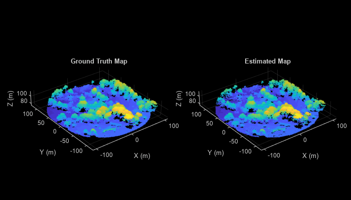
Visualize the ground truth map and the estimated map.

% Create a figure window to display both the ground truth map and estimated map
hFigMap = figure(Position=[0 0 700 400]);
axMap1 = subplot(1,2,1,Color='black',Parent=hFigMap);
axMap1.Position = [0.08 0.2 0.4 0.55];
pcshow(orgMap,Parent=axMap1)
axis on
xlabel(axMap1,'X (m)')
ylabel(axMap1,'Y (m)')
zlabel(axMap1,'Z (m)')
title(axMap1,'Ground Truth Map')

axMap2 = subplot(1,2,2,Color='black',Parent=hFigMap);
axMap2.Position = [0.56 0.2 0.4 0.55];
pcshow(globalMap,Parent=axMap2)
axis on
xlabel(axMap2,'X (m)')
ylabel(axMap2,'Y (m)')
zlabel(axMap2,'Z (m)')
title(axMap2,'Estimated Map')

Figure contains 2 axes objects. Axes object 1 with title Ground Truth Map, xlabel X (m), ylabel Y (m) contains an object of type scatter. Axes object 2 with title Estimated Map, xlabel X (m), ylabel Y (m) contains an object of type scatter.

References

[1] Starr, Scott. "Tuscaloosa, AL: Seasonal Inundation Dynamics and Invertebrate Communities." National Center for Airborne Laser Mapping, December 1, 2011. OpenTopography(https://doi.org/10.5069/G9SF2T3K).