addRelativePose
Add relative pose to pose graph
Syntax
Description
addRelativePose(
creates a node based on the input poseGraph,measurement)measurement that connects to
the last pose node in the pose graph. To add landmark nodes, see the
addPointLandmark function.
addRelativePose(
also specifies the information matrix as part of the edge constraint, which
represents the uncertainty of the pose measurement.poseGraph,measurement,infoMat)
addRelativePose(
creates a new pose node and connects it to the specific node specified by
poseGraph,measurement,infoMat,fromNodeID)fromNodeID.
addRelativePose(
creates an edge by specifying a relative pose measurement between existing nodes
specified by poseGraph,measurement,infoMat,fromNodeID,toNodeID)fromNodeID and toNodeID. This
edge is called a loop closure. If a loop closure already
exists, the function appends the new measurement. Calling the optimizePoseGraph function combines multiple appended measurements
into a single edge. This syntax does not support adding edges to a landmark
node.
Examples
This example shows how to identify and remove spurious loop closures from pose graph. To do this, you can modify the relative pose of a loop closure edge and try optimizing the pose graph with and without removing the auto spurious loop closure and compare the results.
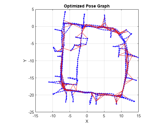
Load the Intel Research Lab Dataset that contains a 2-D pose graph. Optimize the pose graph. Plot the pose graph with IDs off. Red lines indicate loop closures identified in the dataset.
load intel-2d-posegraph.mat pg
optimizedPG = optimizePoseGraph(pg);
show(optimizedPG,IDs="off");
title("Optimized Pose Graph")
Modify the relative pose of the loop closure edge 1386 to some random values.
loopclosureId = 1386;
nodePair = edgeNodePairs(optimizedPG,loopclosureId);
[relPose,infoMat] = edgeConstraints(optimizedPG,loopclosureId);
relPose(2) = -5;
relPose(3) = 1.5;
addRelativePose(optimizedPG,relPose,infoMat,nodePair(1),nodePair(2));
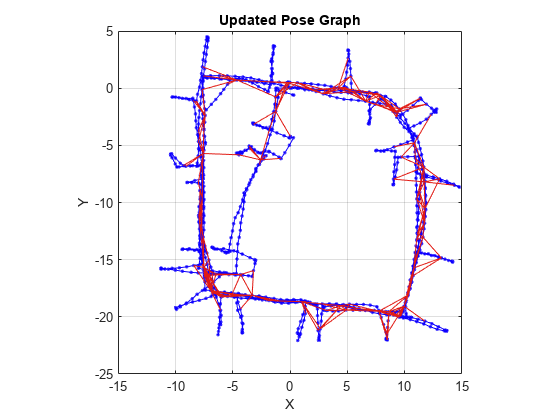
Optimize the pose graph without auto loop closure trimming. Plot the optimized pose graph to see the poor adjustment of the nodes with loop closures.
[updatedPG,solutionInfo] = optimizePoseGraph(optimizedPG);
show(updatedPG,IDs="off");
title("Updated Pose Graph")
Certain loop closures should be trimmed from the pose graph. Use the trimLoopClosures function to trim these bad loop closures. Set the truncation threshold and maximum iterations for the trimmer parameters.
trimParams = struct("TruncationThreshold",0.5,"MaxIterations",100);
Generate solver options.
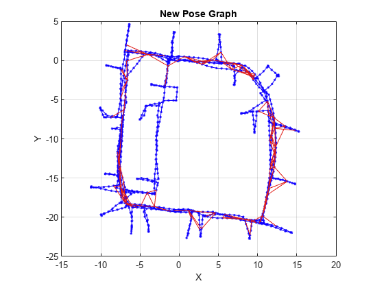
solverOptions = poseGraphSolverOptions("g2o-levenberg-marquardt");Use the trimLoopClosures function with the trimmer parameters and solver options. Plot the new pose graph to see the bad loop closures were removed.
[newPG,trimInfo] = trimLoopClosures(updatedPG,trimParams,solverOptions);
show(newPG,IDs="off");
title("New Pose Graph")
Input Arguments
Output Arguments
Extended Capabilities
Version History
Introduced in R2019b