Landmark SLAM Using AprilTag Markers
This example shows how to combine robot odometry data and observed fiducial markers called AprilTags to better estimate the robot trajectory and the landmark positions in the environment. The example uses a pose graph approach and a factor graph approach, and compares the two graphs.
Download Data Set and Load Sensor Data
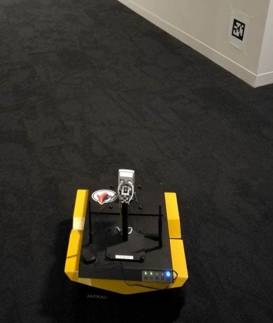
Download a .zip file that contains raw data recorded from a rosbag on a ClearPath Robotics™ Jackal™. The raw data includes:
Images taken using an Axis™ M1013 network camera at a resolution of 640-by-480.
Odometry data preprocessed and synchronized with the image data.
Unzip the file, which contains the data set as a rosbag file and as a .mat file. You can use the exampleHelperExtractDataFromRosbag helper function, provided at the end of this example, to see how the data has been extracted from the rosbag and preprocessed. To use the helper function, you must have a ROS Toolbox license.
filename = matlab.internal.examples.downloadSupportFile("spc/robotics","apriltag_odometry_slam_dataset.zip");
unzip(filename)
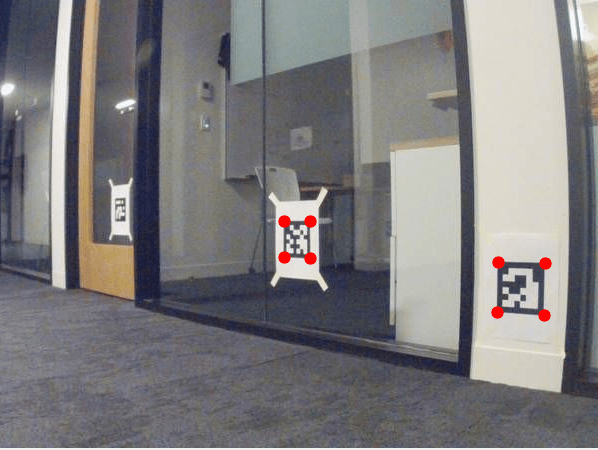
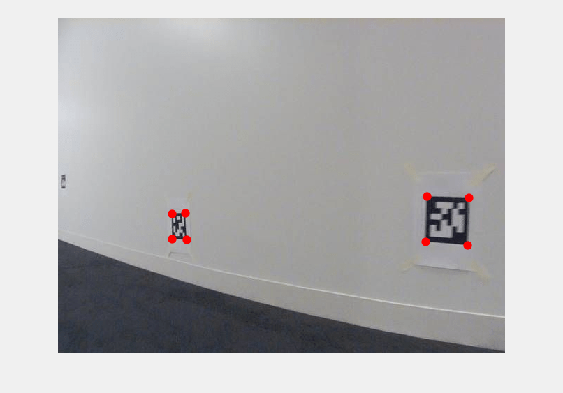
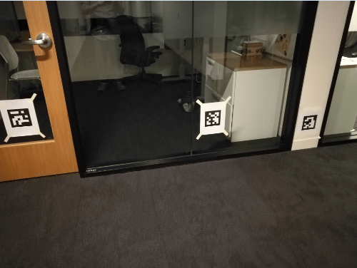
In this example, a set of AprilTag markers have been printed and randomly placed in the test environment. The pose graph and factor graphs treat the tags as landmarks, which are distinguishable features of the environment that enable you to localize with more accuracy. By using the camera intrinsics and the size of each marker, you can convert the images with AprilTag observations into point landmark measurements using the readAprilTag (Computer Vision Toolbox) function. These landmark measurements are relative to the current robot frame. This example includes the camera intrinsic parameters in the cameraParams.mat file, but to determine the intrinsic parameters of your own camera, follow the steps in the Camera Calibration Using Custom Planar Calibration Patterns (Computer Vision Toolbox) example, or use a checkerboard pattern with the Camera Calibrator (Computer Vision Toolbox) app. The AprilTag markers used in this example are from the "tag46h11" family, with no duplicate IDs. The size of the printed tag is 136.65 mm.
tagFamily = "tag36h11";
tagSize = 136.65; % mm
Load the sensor data and camera parameters into the MATLAB® workspace.
load apriltag_odometry_slam_dataset/apriltag_odometry_slam_dataset.mat
load cameraParams.mat
Create an empty dictionary data structure to maintain the mapping between tag IDs and their node IDs.
tagToNodeIDDic = dictionary([],[]);
The sensors recorded the odometry data in the .mat file from the odometry frame to the laser frame that moves with the robot. Apply a fixed transformation between the laser frame and the camera frame.
R1 = [0 0 1; -1 0 0; 0 -1 0];
Ta = blkdiag(R1,1); % The camera frame z-axis points forward and y-axis points down
Tb = eye(4);
T2(1,3) = -0.11;
T(3,3) = 0.146; % Fixed translation of camera frame origin to 'laser' frame
Build Pose Graph from Sensor Data
After importing the synchronized sensor data and the camera parameters, build a 3-D pose graph of node estimates from the measurements in the sensor data. The pose graph contains node estimates, edge contraints, and loop closures that estimate robot poses.
First create the pose graph.
pg = poseGraph3D;
By using fiducial markers like AprilTags, the block pattern in the image provides unique IDs for each landmark observation. This ID information reduces the need for difficult data association algorithms when performing simultaneous localization and mapping (SLAM).
Create a variable to store the previous pose and node ID.
lastTform = [];
lastPoseNodeId = 1;
Create variables to store all the landmark node IDs.
lmkIDs = [];
This example estimates the robot trajectory based on the pose measurements from the odometery data and landmark measurements from the AprilTag observations. Iterate through the sensor data and follow these steps:
Add odometry data to the pose graph using the
addRelativePosefunction. Compute the relative poses between each odometry before adding it to the pose graph.Add landmark measurements from the AprilTag observations in the images using the
readAprilTagfunction. Because an image can contain multiple tags, iterate through all the IDs returned. Add point landmarks relative to the current pose node using theaddPointLandmarkfunction.Show the image with markers around the AprilTag observations. The image updates as you iterate through the data.
figure(Visible="on")
for i = 1:numel(imageData)

    % Add odometry data to pose graph
    T = odomData{i};
    if isempty(lastTform)
        nodePair = addRelativePose(pg,[0 0 0 1 0 0 0],[],lastPoseNodeId);
    else
        relPose = exampleHelperComputeRelativePose(lastTform,T);
        nodePair = addRelativePose(pg,relPose,[],lastPoseNodeId);
    end
    currPoseNodeId = nodePair(2);

    % Add landmark measurement based on AprilTag observation in the image.
    I = imageData{i};
    [id,loc,poseRigid3d,detectedFamily] = readAprilTag(I,tagFamily,cameraParams.Intrinsics,tagSize);

    for j = 1:numel(id)
        % Insert observation markers to image.
        markerRadius = 6;
        numCorners = size(loc,1);
        markerPosition = [loc(:,:,j) repmat(markerRadius,numCorners,1)];
        I = insertShape(I,FilledCircle=markerPosition,Color="red",Opacity=1);

        t = poseRigid3d(j).Translation/1000; % change from mm to meters
        po = [t(:); 1];
        p = Tb*Ta*po;

        if isKey(tagToNodeIDDic,id(j))
            lmkNodeId = tagToNodeIDDic(id(j));
            if ~ismember(lmkNodeId,lmkIDs)
                lmkIDs = [lmkIDs lmkNodeId]; % store unique landmark IDs
            end
            addPointLandmark(pg,p(1:3)',[],currPoseNodeId,lmkNodeId);
        else
            nodePair = addPointLandmark(pg,p(1:3)',[],currPoseNodeId);
            tagToNodeIDDic(id(j)) = nodePair(2);
        end
    end

    % Show the image with AprilTag observation markers.
    imshow(I)
    drawnow

    lastTform = T;
    lastPoseNodeId = currPoseNodeId;
end
Optimize Pose Graph and Inspect Results
After building the pose graph, optimize it using the optimizePoseGraph function.
pgUpd = optimizePoseGraph(pg);
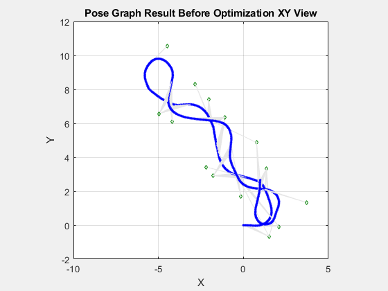
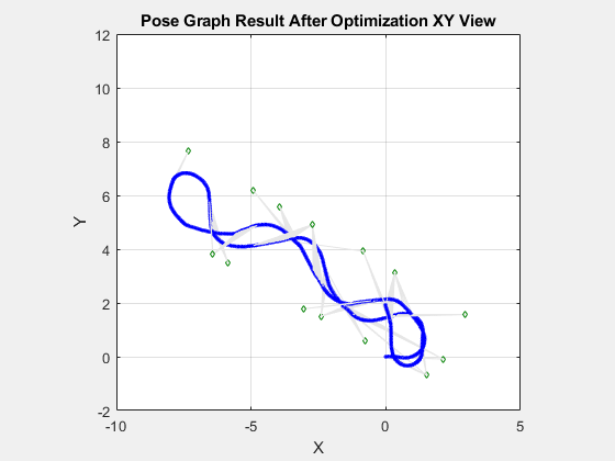
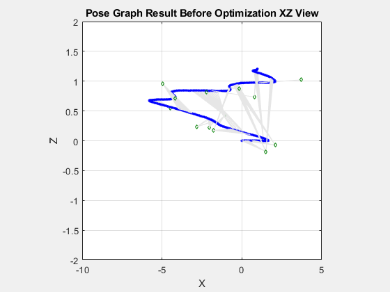
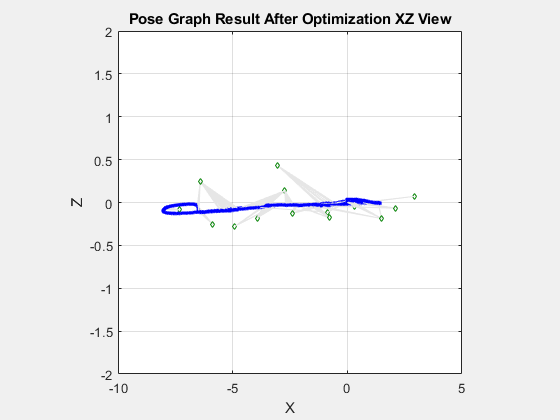
Visualize both the initial and optimized pose graph. The optimized pose graph shows these improvements:
The initial position of the robot relative to the landmarks has been corrected.
The landmarks on each wall are better aligned.
The vertical drift in the robot trajectory along the z-direction has been corrected.
figure(Visible="on")
show(pg);
axis equal
xlim([-10.0 5.0])
ylim([-2.0 12.0])
title("Pose Graph Result Before Optimization XY View")
figure(Visible="on")
show(pgUpd);
axis equal
xlim([-10.0 5.0])
ylim([-2.0 12.0])
title("Pose Graph Result After Optimization XY View")
% Vertical drift.
figure(Visible="on")
show(pg);
axis square
xlim([-10.0 5.0])
zlim([-2.0 2.0])
view(0,0)
title("Pose Graph Result Before Optimization XZ View")
show(pgUpd);
axis square
xlim([-10.0 5.0])
zlim([-2.0 2.0])
view(0,0)
title("Pose Graph Result After Optimization XZ View")
Build Factor Graph from Sensor Data
Alternatively, you can build a factor graph based on the measurements in the sensor data. Using a factor graph makes it easier to include additional sensors in the optimization, and also optimizes faster than the pose graph even though it may take longer to set up and build.
Create the factor graph as a factorGraph object.
G = factorGraph;
Create variables to store the previous pose and node ID.
lastTform = [];
lastPoseNodeId = 1;
tagToNodeIDDic = dictionary([],[]);
Iterate through the sensor data and follow these steps to add factors to the factor graph:
Add odometry data to the factor graph as a factor by relating poses using the
factorTwoPoseSE3object. Compute the relative poses between each odometry before adding it to the factor graph.Add landmark measurements from the AprilTag observations in the images using the
readAprilTagfunction. Because image can contain multiple tags, iterate through all the IDs returned. Add point landmarks relative to the current pose node using thefactorPoseSE3AndPointXYZobject.Show the image with markers around the AprilTag observations. The image updates as you iterate through the data.
for i = 1:numel(imageData)

    % Add odometry data to factor graph
    T = odomData{i};
    if isempty(lastTform)
        % Add a prior factor to loosely fix the initial node at the origin
        fPrior = factorPoseSE3Prior(1);
        addFactor(G,fPrior);
        newPoseNodeId = lastPoseNodeId + 1;
        % The measurement represents a relative pose in SE(3) between lastPoseNode and newPoseNode.
        fctr = factorTwoPoseSE3([lastPoseNodeId newPoseNodeId],Measurement=[0 0 0 1 0 0 0]);
        addFactor(G,fctr);
    else
        % Calculate relative pose between nodes of lastPoseNodeId and newPoseNodeId
        relPose = exampleHelperComputeRelativePose(lastTform,T);
        newPoseNodeId = G.NumNodes + 1;
        fctr = factorTwoPoseSE3([lastPoseNodeId newPoseNodeId],Measurement=relPose);
        addFactor(G,fctr);
    end
    currPoseNodeId = newPoseNodeId;

    % Add landmark measurement based on AprilTag observation in the image.
    I = imageData{i};
    [id,loc,poseRigid3d,detectedFamily] = readAprilTag(I,tagFamily,cameraParams.Intrinsics,tagSize);

    for j = 1:numel(id)
        % Insert observation markers to image.
        markerRadius = 6;
        numCorners = size(loc,1);
        markerPosition = [loc(:,:,j),repmat(markerRadius,numCorners,1)];
        I = insertShape(I,FilledCircle=markerPosition,Color="red",Opacity=1);

        t = poseRigid3d(j).Translation/1000; % change from mm to meter
        po = [t(:); 1];
        p = Tb*Ta*po;

        if isKey(tagToNodeIDDic,id(j))
            lmkNodeId = tagToNodeIDDic(id(j));
            % The measurement represents a relative position [dx,dy,dz] between landmark point and current pose node.
            fctr = factorPoseSE3AndPointXYZ([currPoseNodeId lmkNodeId],Measurement=p(1:3)');
            addFactor(G,fctr);
        else
            newPointNodeId = G.NumNodes + 1;
            fctr = factorPoseSE3AndPointXYZ([currPoseNodeId newPointNodeId],Measurement=p(1:3)');
            addFactor(G,fctr);
            tagToNodeIDDic(id(j)) = newPointNodeId;
        end
    end

    % Show the image with AprilTag observation markers.
    imshow(I)
    drawnow limitrate

    lastTform = T;
    lastPoseNodeId = currPoseNodeId;
end

Optimize Factor Graph and Inspect Results
After building the factor graph, optimize it using the optimize object function with solver options defined by a factorGraphSolverOptions object. Set the VerbosityLevel property to 2 to show more detail of the optimization process.
opt = factorGraphSolverOptions(VerbosityLevel=2);
soln = optimize(G,opt)
iter      cost      cost_change  |gradient|   |step|    tr_ratio  tr_radius  ls_iter  iter_time  total_time
   0  4.984516e+02    0.00e+00    5.76e+01   0.00e+00   0.00e+00  1.00e+04        0    2.56e-03    6.04e-03
   1  8.515843e+02   -3.53e+02    5.76e+01   7.53e+01  -7.13e-01  5.00e+03        1    1.94e-02    2.70e-02
   2  8.515843e+02   -3.53e+02    5.76e+01   7.53e+01  -7.13e-01  2.50e+03        0    1.06e-03    3.04e-02
   3  8.515843e+02   -3.53e+02    5.76e+01   7.53e+01  -7.13e-01  1.25e+03        0    6.45e-04    3.26e-02
   4  8.515843e+02   -3.53e+02    5.76e+01   7.53e+01  -7.13e-01  6.25e+02        0    7.57e-04    3.54e-02
   5  8.515843e+02   -3.53e+02    5.76e+01   7.53e+01  -7.13e-01  3.12e+02        0    7.01e-04    3.78e-02
   6  8.515843e+02   -3.53e+02    5.76e+01   7.53e+01  -7.13e-01  1.56e+02        0    6.11e-04    3.96e-02
   7  8.515843e+02   -3.53e+02    5.76e+01   7.53e+01  -7.13e-01  7.81e+01        0    6.51e-04    4.14e-02
   8  5.087687e+02   -1.03e+01    5.76e+01   4.26e+01  -2.13e-02  3.91e+01        0    7.57e-04    4.35e-02
   9  1.365586e+02    3.62e+02    3.27e+01   1.99e+01   7.77e-01  1.17e+02        0    3.05e-03    4.68e-02
  10  4.583660e+02   -3.22e+02    3.27e+01   6.72e+01  -2.40e+00  5.86e+01        1    9.06e-03    5.62e-02
  11  5.329830e+01    8.33e+01    1.94e+01   3.35e+01   6.64e-01  5.86e+01        0    4.06e-03    6.06e-02
  12  5.142921e+01    1.87e+00    1.91e+01   3.05e+01   3.72e-02  2.93e+01        1    1.44e-02    7.54e-02
  13  8.811991e+00    4.26e+01    4.56e+00   1.74e+01   9.59e-01  8.79e+01        1    1.11e-02    8.68e-02
  14  1.032690e+02   -9.45e+01    4.56e+00   5.11e+01  -1.23e+01  4.39e+01        1    1.75e-02    1.05e-01
  15  9.869378e+00   -1.06e+00    4.56e+00   2.55e+01  -1.63e-01  2.20e+01        0    9.05e-04    1.06e-01
  16  3.688774e+00    5.12e+00    2.19e+00   1.28e+01   9.18e-01  6.59e+01        0    2.74e-03    1.09e-01
  17  3.409290e+01   -3.04e+01    2.19e+00   3.84e+01  -1.16e+01  3.30e+01        1    8.06e-03    1.17e-01
  18  4.290375e+00   -6.02e-01    2.19e+00   1.92e+01  -3.01e-01  1.65e+01        0    6.80e-04    1.18e-01
  19  2.344156e+00    1.34e+00    1.79e+00   9.61e+00   8.38e-01  4.94e+01        0    2.68e-03    1.21e-01
  20  1.153071e+01   -9.19e+00    1.79e+00   2.88e+01  -6.83e+00  2.47e+01        1    8.27e-03    1.30e-01
  21  2.301715e+00    4.24e-02    3.62e+00   1.44e+01   4.43e-02  1.24e+01        0    2.67e-03    1.33e-01
  22  1.395292e+00    9.06e-01    1.65e+00   7.21e+00   8.84e-01  3.71e+01        1    1.27e-02    1.46e-01
  23  2.835470e+00   -1.44e+00    1.65e+00   2.17e+01  -1.95e+00  1.85e+01        1    1.05e-02    1.59e-01
  24  1.118728e+00    2.77e-01    1.76e+00   1.08e+01   5.51e-01  1.85e+01        0    3.10e-03    1.64e-01
  25  7.683906e-01    3.50e-01    1.50e+00   1.09e+01   7.36e-01  1.85e+01        1    1.11e-02    1.77e-01
  26  5.116551e-01    2.57e-01    9.30e-01   1.10e+01   7.67e-01  5.56e+01        1    1.31e-02    1.92e-01
  27  3.957137e+00   -3.45e+00    9.30e-01   3.31e+01  -8.79e+00  2.78e+01        1    1.04e-02    2.04e-01
  28  4.955209e-01    1.61e-02    1.77e+00   1.65e+01   5.60e-02  1.39e+01        0    2.89e-03    2.08e-01
  29  2.135810e-01    2.82e-01    7.81e-01   8.27e+00   8.94e-01  4.17e+01        1    1.15e-02    2.21e-01
  30  1.599750e+00   -1.39e+00    7.81e-01   2.17e+01  -9.94e+00  2.09e+01        1    1.26e-02    2.35e-01
  31  2.592216e-01   -4.56e-02    7.81e-01   1.23e+01  -3.75e-01  1.04e+01        0    1.46e-03    2.39e-01
  32  1.358879e-01    7.77e-02    2.36e-01   6.16e+00   8.56e-01  3.13e+01        0    4.65e-03    2.44e-01
  33  8.608814e-01   -7.25e-01    2.36e-01   1.57e+01  -1.11e+01  1.56e+01        1    8.79e-03    2.53e-01
  34  1.788477e-01   -4.30e-02    2.36e-01   9.13e+00  -7.68e-01  7.82e+00        0    5.21e-04    2.54e-01
  35  1.064787e-01    2.94e-02    3.08e-01   4.56e+00   7.69e-01  2.35e+01        0    2.57e-03    2.56e-01
  36  4.251862e-01   -3.19e-01    3.08e-01   1.12e+01  -8.44e+00  1.17e+01        1    1.49e-02    2.71e-01
  37  1.229167e-01   -1.64e-02    3.08e-01   6.74e+00  -4.99e-01  5.87e+00        0    5.38e-04    2.72e-01
  38  8.755732e-02    1.89e-02    1.78e-01   3.37e+00   8.22e-01  1.76e+01        0    4.46e-03    2.77e-01
  39  2.110173e-01   -1.23e-01    1.78e-01   8.08e+00  -6.32e+00  8.80e+00        1    1.31e-02    2.91e-01
  40  9.263937e-02   -5.08e-03    1.78e-01   4.98e+00  -2.96e-01  4.40e+00        0    1.05e-03    2.92e-01
  41  7.771281e-02    9.84e-03    1.22e-01   2.49e+00   8.35e-01  1.32e+01        0    4.50e-03    2.97e-01
  42  1.160680e-01   -3.84e-02    1.22e-01   5.86e+00  -3.85e+00  6.60e+00        1    1.26e-02    3.10e-01
  43  7.727460e-02    4.38e-04    3.67e-01   3.70e+00   4.96e-02  3.30e+00        0    4.57e-03    3.15e-01
  44  6.863371e-02    8.64e-03    1.28e-01   1.90e+00   9.32e-01  9.90e+00        1    1.67e-02    3.32e-01
  45  6.766036e-02    9.73e-04    2.30e-02   1.25e+00   9.83e-01  9.90e+00        1    1.34e-02    3.46e-01
  46  6.764183e-02    1.85e-05    8.05e-05   9.00e-02   1.00e+00  9.90e+00        1    1.26e-02    3.62e-01
Terminating: Function tolerance reached. |cost_change|/cost: 1.078674e-07 <= 1.000000e-06

Solver Summary (v 2.0.0-eigen-(3.3.4)-no_lapack-eigensparse-no_openmp-no_custom_blas)

                                     Original                  Reduced
Parameter blocks                          585                      585
Parameters                               4039                     4039
Effective parameters                     3468                     3468
Residual blocks                           804                      804
Residuals                                4125                     4125

Minimizer                        TRUST_REGION

Sparse linear algebra library    EIGEN_SPARSE
Trust region strategy                  DOGLEG (TRADITIONAL)

                                        Given                     Used
Linear solver          SPARSE_NORMAL_CHOLESKY   SPARSE_NORMAL_CHOLESKY
Threads                                     1                        1
Linear solver ordering              AUTOMATIC                      585

Cost:
Initial                          4.984516e+02
Final                            6.764183e-02
Change                           4.983839e+02

Minimizer iterations                       47
Successful steps                           22
Unsuccessful steps                         25

Time (in seconds):
Preprocessor                         0.003480

  Residual only evaluation           0.021286 (47)
  Jacobian & residual evaluation     0.054238 (22)
  Linear solver                      0.219521 (22)
Minimizer                            0.371506

Postprocessor                        0.000229
Total                                0.375216

Termination:                      CONVERGENCE (Function tolerance reached. |cost_change|/cost: 1.078674e-07 <= 1.000000e-06)
soln = struct with fields:
             InitialCost: 498.4516
               FinalCost: 0.0676
      NumSuccessfulSteps: 22
    NumUnsuccessfulSteps: 25
               TotalTime: 0.3752
         TerminationType: 0
        IsSolutionUsable: 1
        OptimizedNodeIDs: [1 2 3 4 5 6 7 8 9 10 11 12 13 14 15 16 17 18 19 20 21 22 23 24 25 26 27 28 29 30 31 32 33 34 35 36 37 38 39 40 41 42 43 44 45 46 47 48 49 50 51 52 53 54 55 56 57 58 59 60 61 62 63 64 65 66 67 68 69 70 71 72 73 74 75 76 77 … ]
            FixedNodeIDs: [1×0 double]
The returned solution information indicates that the optimize object function has greatly reduced the cost of the path, which indicates that the optimization process has improved the path. The IsSolutionUsable value of 1 also indicates that the solution is viable. If optimize does not return converging results, consider adjusting solver options, such as the number of maximum iterations, depending on the returned cost_change and gradient values for each step.
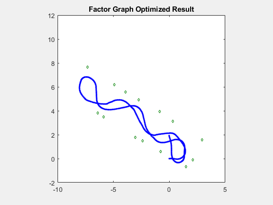
Retrieve the optimized results, and visualize the robot trajectory in blue and landmark points in green.
fgNodeStates = exampleHelperShowFactorGraphResult(G);
Conclusion
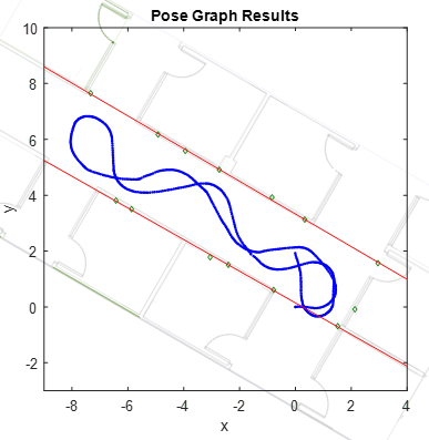
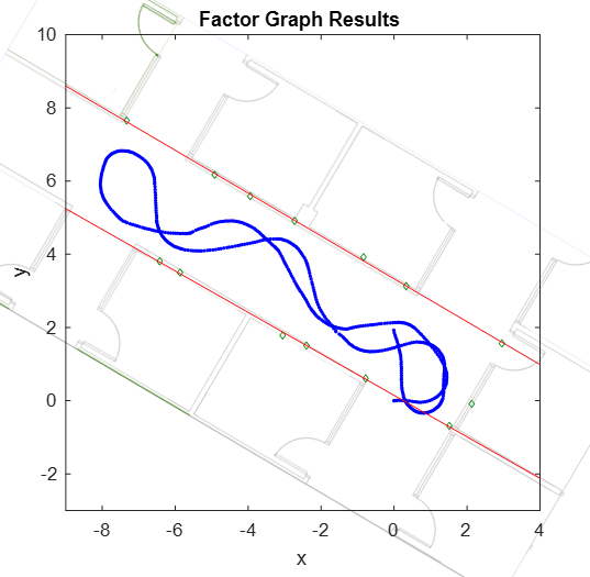
These images show the final robot trajectories, generated by the pose graph and factor graph, overlaid on the blueprint of the office area using a transformation to show the accuracy of the estimated trajectory and the estimated landmark locations. If you play back the images again, you can see a strong correlation between the pose graph and factor graph.. All green landmarks are on or near the walls, and the two fitted lines based on the detected landmarks overlap with the walls of the hallway. However, though these two solutions are visually similar, we can compare them numerically.
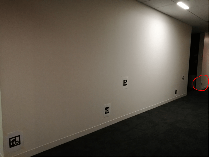
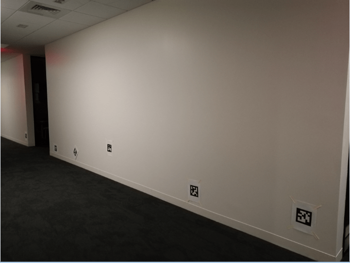
These images show the positions of the AprilTags for your reference. Note that there is one AprilTag that is not picked up by the camera, marked by a red circle.
To numerically compare the difference between the results of the pose graph and the factor graph, retrieve the node states from the updated pose graph, and compute the average absolute difference for robot positions, rotation angles, and landmark positions between it and the factor graph.
pgUpdNodeStates = nodeEstimates(pgUpd);
[robotPosDiff,robotRotDiff,lmkDiff] = exampleHelperComputeDifference(pgUpdNodeStates,fgNodeStates,lmkIDs)
robotPosDiff = 1×3
10-3 ×

    0.0524    0.0924    0.9312
robotRotDiff = 1×3
10-3 ×

    0.0198    0.1625    0.1355
lmkDiff = 1×3
10-3 ×

    0.0562    0.0865    0.8646
Note that, to better compare with pose graph result, you specified an initial guess for the pose of the initial node of the factor graph at the origin by using a factorPoseSE3Prior object. Without the prior factor, the factor graph optimization process results in a graph that has optimal relative poses and positions but the absolute poses, and positions are not necessarily correct. The average absolute difference is fairly small, which means both methods give similar optimized results. Compared to the pose graph, the optimization time of the factor graph is much shorter, but it takes a longer time to set up and build the factor graph.