Main Content

edgeConstraints

Edge constraints in pose graph

Description

measurements = edgeConstraints(poseGraph) lists all edge constraints in the specified pose graph as a relative pose.

[measurements,infoMats] = edgeConstraints(poseGraph) also returns the information matrices for each edge. The information matrix is the inverse of the covariance of the pose measurement.

[measurements,infoMats] = edgeConstraints(poseGraph,edgeIDs) returns edge constraints for the specified edge IDs.

example

Examples

collapse all

This example shows how to identify and remove spurious loop closures from pose graph. To do this, you can modify the relative pose of a loop closure edge and try optimizing the pose graph with and without removing the auto spurious loop closure and compare the results.

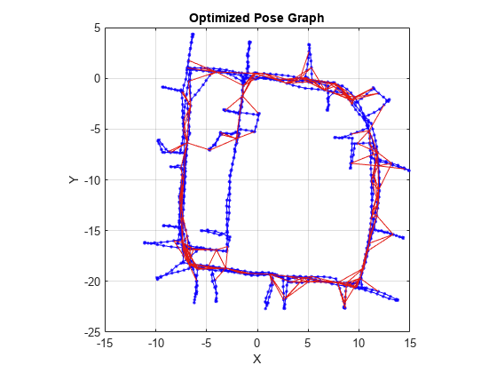
Load the Intel Research Lab Dataset that contains a 2-D pose graph. Optimize the pose graph. Plot the pose graph with IDs off. Red lines indicate loop closures identified in the dataset.

load intel-2d-posegraph.mat pg
optimizedPG = optimizePoseGraph(pg);
show(optimizedPG,IDs="off");
title("Optimized Pose Graph")

Figure contains an axes object. The axes object with title Optimized Pose Graph, xlabel X, ylabel Y contains 3 objects of type line. One or more of the lines displays its values using only markers

Modify the relative pose of the loop closure edge 1386 to some random values.

loopclosureId = 1386;
nodePair = edgeNodePairs(optimizedPG,loopclosureId);
[relPose,infoMat] = edgeConstraints(optimizedPG,loopclosureId);
relPose(2) = -5;
relPose(3) = 1.5;
addRelativePose(optimizedPG,relPose,infoMat,nodePair(1),nodePair(2));

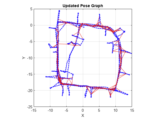
Optimize the pose graph without auto loop closure trimming. Plot the optimized pose graph to see the poor adjustment of the nodes with loop closures.

[updatedPG,solutionInfo] = optimizePoseGraph(optimizedPG);
show(updatedPG,IDs="off");
title("Updated Pose Graph")

Figure contains an axes object. The axes object with title Updated Pose Graph, xlabel X, ylabel Y contains 3 objects of type line. One or more of the lines displays its values using only markers

Certain loop closures should be trimmed from the pose graph. Use the trimLoopClosures function to trim these bad loop closures. Set the truncation threshold and maximum iterations for the trimmer parameters.

trimParams = struct("TruncationThreshold",0.5,"MaxIterations",100);

Generate solver options.

solverOptions = poseGraphSolverOptions("g2o-levenberg-marquardt");

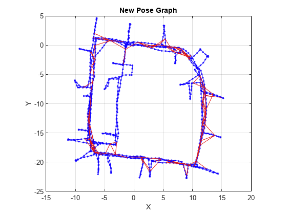
Use the trimLoopClosures function with the trimmer parameters and solver options. Plot the new pose graph to see the bad loop closures were removed.

[newPG,trimInfo] = trimLoopClosures(updatedPG,trimParams,solverOptions);
show(newPG,IDs="off");
title("New Pose Graph")

Figure contains an axes object. The axes object with title New Pose Graph, xlabel X, ylabel Y contains 3 objects of type line. One or more of the lines displays its values using only markers

Input Arguments

collapse all

Pose graph, specified as a poseGraph or poseGraph3D object.

Edge IDs, specified as a vector of positive integers.

Output Arguments

collapse all

Measurements between nodes, returned as an n-by-3 matrix or n-by-7 matrix.

For poseGraph (2-D), each row is an [x y theta] vector, which defines the relative xy-position and orientation angle, theta, of a pose in the graph. For landmark positions, theta is returned as NaN.

For poseGraph3D, each row is an [x y z qw qx qy qz] vector, which defines the relative xyz-position and quaternion orientation, [qw qx qy qz], of a pose in the graph.

Note

Many other sources for 3-D pose graphs, including .g2o formats, specify the quaternion orientation in a different order, for example, [qx qy qz qw]. Check the source of your pose graph data before adding nodes to your poseGraph3D object.

Information matrices, specified in compact form as a n-by-6 or n-by-21 matrix, where n is the number of poses in the pose graph.

Each row is the upper triangle of the square information matrix. An information matrix represents the uncertainty of the measurement. The matrix is calculated as the inverse of the covariance. If the measurement is an [x y theta] vector, the covariance matrix is a 3-by-3 of pairwise covariance calculations. Typically, the uncertainty is determined by the sensor model.

For poseGraph (2-D), each information matrix is a six-element vector. The default is [1 0 0 1 0 1]. For landmark nodes, the last three elements are returned as NaN.

For poseGraph3D, each information matrix is a 21-element vector. The default is [1 0 0 0 0 0 1 0 0 0 0 1 0 0 0 1 0 0 1 0 1].

Extended Capabilities

Version History

Introduced in R2019b