Linear Regression with Multiple Predictor Variables
Multiple linear regression describes the relationship between two or more predictor variables and a response variable. Multiple linear regression models are useful when the response depends on several factors and you want to understand how each factor contributes to the outcome.
This example shows how to fit a multiple linear regression model by building a design matrix and using the backslash operator (\) (mldivide function). This example also shows how to evaluate and validate the model. For information about fitting and visualizing a model using the Basic Fitting tool instead, see Interactively Fit Data and Visualize Model.
Use multiple linear regression when:
You have two or more predictor variables.
The relationship between the predictors and the response is linear in the coefficients.
You want to quantify the effect of each predictor on the response.
Construct Design Matrix
First, create two sample predictor variables factor1 and factor2 and a sample response variable outcome.
n = 40;
factor1 = 1 + 4*rand(n,1);
factor2 = 4 + 6*rand(n,1);
outcome = 20 + 8*factor1 + 4*factor2 - factor1.*factor2 + 2*randn(n,1);
A design matrix organizes the predictor variables for your data. Each row in the design matrix corresponds to a data point, and each column corresponds to a predictor term.
For this example with two predictor variables, include these terms in the design matrix:
Column 1 — Intercept for the constant term
Column 2 — First predictor variable
Column 3 — Second predictor variable
This design matrix represents the equation . For your own data, include one term for each predictor variable, and optionally include terms for the interactions between the predictor variables.
numObservations = numel(factor1);
X = [ones(numObservations,1) factor1 factor2 factor1.*factor2];
Fit Model
Fit the regression model by solving for the coefficients that minimize the least-squares error by using the \ operator with the design matrix and response data.
p = X\outcome
p = 4×1

   22.1184
    8.6200
    3.6672
   -1.0772
Define an anonymous function that predicts the outcome for predictor variable values that you specify.
predictOutcome = @(factor1,factor2) p(1) + p(2).*factor1 + p(3)*factor2 + p(4)*factor1.*factor2
predictOutcome = function_handle with value:
    @(factor1,factor2)p(1)+p(2).*factor1+p(3)*factor2+p(4)*factor1.*factor2
Evaluate and Visualize Model
Use the model to predict the outcome for a grid of possible values of the predictor variables.
factor1fit = linspace(min(factor1), max(factor1), 30);
factor2fit = linspace(min(factor2), max(factor2), 30);
[factor1grid, factor2grid] = meshgrid(factor1fit,factor2fit);
gridOutcome = predictOutcome(factor1grid,factor2grid);
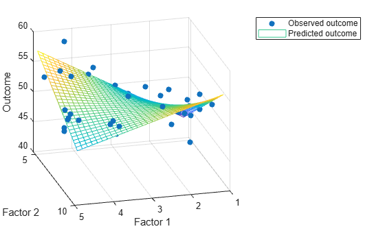
Visualize the observed outcomes and the outcomes predicted by the model on a 3-D plot.
scatter3(factor1,factor2,outcome,"filled")
hold on
mesh(factor1grid,factor2grid,gridOutcome)
hold off

xlabel("Factor 1")
ylabel("Factor 2")
zlabel("Outcome")
view(165,25)
legend("Observed outcome","Predicted outcome")
Validate Model
To validate the model, compute the largest error between the outcomes predicted by the model and the observed outcomes for the same combinations of predictor variables. A small error relative to the outcomes indicates a good fit.
sampleOutcome = predictOutcome(factor1,factor2)
sampleOutcome = 40×1

   52.7253
   53.7132
   52.6716
   50.4299
   51.8525
   49.1566
   49.6175
   51.4355
   51.0745
   50.6402
   46.9813
   51.3436
   51.5744
   49.9553
   54.2865
      ⋮
maxError = max(abs(sampleOutcome - outcome))
maxError =
4.7744
See Also
Functions
Topics
- Linear Regression with One Predictor Variable
- Linear Regression with Nonpolynomial Terms
- Create and Evaluate Polynomials
- Linear Regression Workflow (Statistics and Machine Learning Toolbox)
- Fit Polynomial Models (Curve Fitting Toolbox)