Polynomial Models

About Polynomial Models

Polynomial models for curves are given by

$y = \sum_{i = 1}^{n + 1} p_{i} x^{n + 1 - i}$

where n + 1 is the order of the polynomial, n is the degree of the polynomial, and 1 ≤ n ≤ 9. The order gives the number of coefficients to be fit, and the degree gives the highest power of the predictor variable.

In this guide, polynomials are described in terms of their degree. For example, a third-degree (cubic) polynomial is given by

$γ = p_{1} x^{3} + p_{2} x^{2} + p_{3} x + p_{4}$

Polynomials are often used when a simple empirical model is required. You can use the polynomial model for interpolation or extrapolation, or to characterize data using a global fit. For example, the temperature-to-voltage conversion for a Type J thermocouple in the 0 to 760^o temperature range is described by a seventh-degree polynomial.

Note

If you do not require a global parametric fit and want to maximize the flexibility of the fit, piecewise polynomials might provide the best approach. Refer to Nonparametric Fitting for more information.

The main advantages of polynomial fits include reasonable flexibility for data that is not too complicated, and they are linear, which means the fitting process is simple. The main disadvantage is that high-degree fits can become unstable. Additionally, polynomials of any degree can provide a good fit within the data range, but can diverge wildly outside that range. Therefore, exercise caution when extrapolating with polynomials.

When you fit with high-degree polynomials, the fitting procedure uses the predictor values as the basis for a matrix with very large values, which can result in scaling problems. To handle this, you should normalize the data by centering it at zero mean and scaling it to unit standard deviation. Normalize data by selecting the Center and scale check box in the Curve Fitter app.

Fit Polynomial Models Interactively

Open the Curve Fitter app by entering curveFitter at the MATLAB^® command line. Alternatively, on the Apps tab, in the Math, Statistics and Optimization group, click Curve Fitter.
In the Curve Fitter app, select curve or surface data. On the Curve Fitter tab, in the Data section, click Select Data. Select data variables in the dialog box.
- If you select curve data (X data and Y data, or just Y data against an index), the Curve Fitter app creates the default curve fit, which is a Polynomial fit.
- If you select surface data (X data, Y data, and Z data), the Curve Fitter app creates the default surface fit, which is an Interpolant fit. Click the arrow in the Fit Type section to open the gallery, and click Polynomial in the Regression Models group.

For curve data, the app creates a Polynomial fit for X.

Fit Options pane for curve data polynomial fit

For surface data, the app creates a Polynomial fit for X and Y.

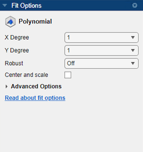
Fit Options pane for surface data polynomial fit

You can specify the following options in the Fit Options pane:

The degree for the X and Y variables:
- For curve data, the degree of X can be up to 9.
- For surface data, the degree of X and Y can be up to 5. The degree of the Polynomial fit is the maximum of X and Y degrees. For more information, see Defining Polynomial Terms for Polynomial Surface Fits.
The robust linear least-squares fitting method to use (Off, LAR, or Bisquare). For details, see the Robust name-value argument of the fitoptions function.
Set bounds or exclude terms. You can exclude any term by setting its bounds to 0. Look in the Results pane to see the model terms, the values of the coefficients, and the goodness-of-fit statistics.

Tip

If your data variables have very different scales, select and clear the Center and scale check box to see the difference in the fit. The app displays messages in the Results pane when scaling the data can improve the fit.

For an example comparing various polynomial fits, see Compare Fits in Curve Fitter App.

Fit Polynomials Using the Fit Function

Open Live Script

This example shows how to use the fit function to fit polynomials to data. The steps fit and plot polynomial curves and a surface, specify fit options, return goodness of fit statistics, calculate predictions, and show confidence intervals.

The polynomial library model is an input argument to the fit and fittype functions. Specify the model type poly followed by the degree in x (up to 9), or x and y (up to 5). For example, you specify a quadratic curve with 'poly2' , or a cubic surface with 'poly33'.

Create and Plot a Quadratic Polynomial Curve

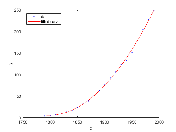
Load some data and fit a quadratic polynomial. Specify a quadratic, or second-degree polynomial, with the string 'poly2'.

load census
fitpoly2 = fit(cdate,pop,'poly2')

fitpoly2 = 
     Linear model Poly2:
     fitpoly2(x) = p1*x^2 + p2*x + p3
     Coefficients (with 95% confidence bounds):
       p1 =    0.006541  (0.006124, 0.006958)
       p2 =      -23.51  (-25.09, -21.93)
       p3 =   2.113e+04  (1.964e+04, 2.262e+04)

% Plot the fit with the plot method.
plot(fitpoly2,cdate,pop)
% Move the legend to the top left corner.
legend('Location','NorthWest');

Figure contains an axes object. The axes object with xlabel x, ylabel y contains 2 objects of type line. One or more of the lines displays its values using only markers These objects represent Data, Fitted curve.

Create a Cubic Curve

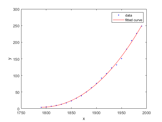
Fit a cubic polynomial 'poly3'.

fitpoly3 = fit(cdate,pop,'poly3')

Warning: Equation is badly conditioned. Try centering and scaling, or add points at non-repeated x values.

fitpoly3 = 
     Linear model Poly3:
     fitpoly3(x) = p1*x^3 + p2*x^2 + p3*x + p4
     Coefficients (with 95% confidence bounds):
       p1 =   3.855e-06  (-4.078e-06, 1.179e-05)
       p2 =    -0.01532  (-0.06031, 0.02967)
       p3 =       17.78  (-67.2, 102.8)
       p4 =       -4852  (-5.834e+04, 4.863e+04)

plot(fitpoly3,cdate,pop)

Specify Fit Options

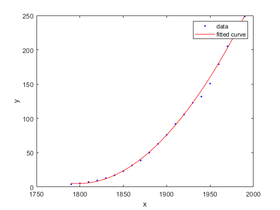
The cubic fit warns that the equation is badly conditioned, so you should try centering and scaling by specifying the 'Normalize' option. Fit the cubic polynomial with both center and scale and robust fitting options. Robust 'on' is a shortcut equivalent to 'Bisquare' , the default method for robust linear least-squares fitting method.

fit3 = fit(cdate, pop,'poly3','Normalize','on','Robust','on')

fit3 = 
     Linear model Poly3:
     fit3(x) = p1*x^3 + p2*x^2 + p3*x + p4
       where x is normalized by mean 1890 and std 62.05
     Coefficients (with 95% confidence bounds):
       p1 =     -0.4619  (-1.895, 0.9707)
       p2 =       25.01  (23.79, 26.22)
       p3 =       77.03  (74.37, 79.7)
       p4 =       62.81  (61.26, 64.37)

plot(fit3,cdate,pop)

To find out what parameters you can set for the library model 'poly3' , use the fitoptions function.

fitoptions poly3

ans = 
  llsqoptions with properties:

        Lower: []
        Upper: []
       Robust: 'Off'
    Normalize: 'off'
      Exclude: []
      Weights: []
       Method: 'LinearLeastSquares'

Get Goodness of Fit Statistics

Specify the 'gof' output argument to get the goodness-of-fit statistics for the cubic polynomial fit.

[fit4, gof] = fit(cdate,pop,'poly3','Normalize','on');
gof

gof = struct with fields:
           sse: 149.7687
       rsquare: 0.9988
           dfe: 17
    adjrsquare: 0.9986
          rmse: 2.9682

Plot the Residuals to Evaluate the Fit

To plot residuals, specify 'residuals' as the plot type in the plot method.

plot(fit4,cdate, pop,'residuals');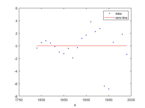

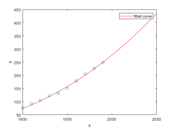
Figure contains an axes object. The axes object with xlabel x contains 2 objects of type line. One or more of the lines displays its values using only markers These objects represent Data, Zero line.

Examine a Fit Beyond the Data Range

By default, the fit is plotted over the range of the data. To plot a fit over a different range, set the x-limits of the axes before plotting the fit. For example, to see values extrapolated from the fit, set the upper x-limit to 2050.

plot(cdate,pop,'o');
xlim([1900, 2050]);
hold on
plot(fit4);
hold off

Figure contains an axes object. The axes object with xlabel x, ylabel y contains 2 objects of type line. One or more of the lines displays its values using only markers This object represents Fitted curve.

Plot Prediction Bounds

To plot prediction bounds, use 'predobs' or 'predfun' as the plot type.

plot(fit4,cdate,pop,'predobs')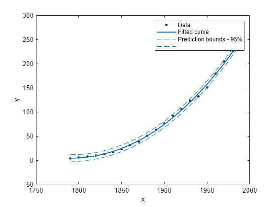

Figure contains an axes object. The axes object with xlabel x, ylabel y contains 4 objects of type line. One or more of the lines displays its values using only markers These objects represent Data, Fitted curve, Prediction bounds - 95%.

Plot prediction bounds for the cubic polynomial up to year 2050.

plot(cdate,pop,'o');
xlim([1900, 2050])
hold on
plot(fit4,'predobs');
hold off

Get Confidence Bounds at New Query Points

Evaluate the fit for some new query points.

cdateFuture = (2000:10:2020).';
popFuture = fit4( cdateFuture )

popFuture = 3×1

  276.9632
  305.4420
  335.5066

Compute 95% confidence bounds on the prediction for the population in the future, using the predint method.

ci = predint(fit4,cdateFuture,0.95,'observation')

ci = 3×2

  267.8589  286.0674
  294.3070  316.5770
  321.5924  349.4208

Plot the predicted future population, with confidence intervals, against the fit and data.

plot(cdate, pop, 'o');
xlim([1900, 2040])
hold on
plot(fit4)
h = errorbar(cdateFuture,popFuture,popFuture-ci(:,1),ci(:,2)-popFuture,'.');
hold off
legend('cdate v pop','poly3','prediction','Location','NorthWest')

Figure contains an axes object. The axes object with xlabel x, ylabel y contains 3 objects of type line, errorbar. One or more of the lines displays its values using only markers These objects represent cdate v pop, poly3, prediction.

Fit and Plot a Polynomial Surface

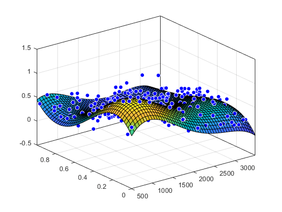
Load some surface data and fit a fourth-degree polynomial in x and y.

load franke
fitsurface = fit([x,y],z, 'poly44','Normalize','on')

fitsurface = 
     Linear model Poly44:
     fitsurface(x,y) = p00 + p10*x + p01*y + p20*x^2 + p11*x*y + p02*y^2 + p30*x^3 
                    + p21*x^2*y + p12*x*y^2 + p03*y^3 + p40*x^4 + p31*x^3*y 
                    + p22*x^2*y^2 + p13*x*y^3 + p04*y^4
       where x is normalized by mean 1982 and std 868.6
       and where y is normalized by mean 0.4972 and std 0.2897
     Coefficients (with 95% confidence bounds):
       p00 =      0.3471  (0.3033, 0.3909)
       p10 =     -0.1502  (-0.1935, -0.107)
       p01 =     -0.4203  (-0.4637, -0.377)
       p20 =      0.2165  (0.1514, 0.2815)
       p11 =      0.1717  (0.1175, 0.2259)
       p02 =     0.03189  (-0.03351, 0.09729)
       p30 =     0.02778  (0.00749, 0.04806)
       p21 =     0.01501  (-0.002807, 0.03283)
       p12 =    -0.03659  (-0.05439, -0.01879)
       p03 =      0.1184  (0.09812, 0.1387)
       p40 =    -0.07661  (-0.09984, -0.05338)
       p31 =    -0.02487  (-0.04512, -0.004624)
       p22 =   0.0007464  (-0.01948, 0.02098)
       p13 =    -0.02962  (-0.04987, -0.009366)
       p04 =    -0.02399  (-0.0474, -0.0005797)

plot(fitsurface,[x,y],z)

Figure contains an axes object. The axes object contains 2 objects of type line, surface. One or more of the lines displays its values using only markers

Polynomial Model Fit Options

All fitting methods have the default propertiesNormalize, Exclude, Weights, and Method. For an example, see Specify Fit Options at the Command Line.

Polynomial models have the Method property value LinearLeastSquares, and the additional fit options properties shown in the next table. For details on all fit options, see the fitoptions reference page.

Property	Description
`Robust`	Specifies the robust linear least-squares fitting method to use. Values are `'on'`, `'off'`, `'LAR'`, or `'Bisquare'`. The default is `'off'`. `'LAR'` specifies the least absolute residual method and `'Bisquare'` specifies the bisquare weights method. `'on'` is equivalent to `'Bisquare'`, the default method.
`Lower`	A vector of lower bounds on the coefficients to be fitted. The default value is an empty vector, indicating that the fit is unconstrained by lower bounds. If bounds are specified, the vector length must equal the number of coefficients. Individual unconstrained lower bounds can be specified by `-Inf`.
`Upper`	A vector of upper bounds on the coefficients to be fitted. The default value is an empty vector, indicating that the fit is unconstrained by upper bounds. If bounds are specified, the vector length must equal the number of coefficients. Individual unconstrained upper bounds can be specified by `Inf`.

Defining Polynomial Terms for Polynomial Surface Fits

You can control the terms to include in the polynomial surface model by specifying the degrees for the x and y inputs. If i is the degree in x and j is the degree in y, the total degree of the polynomial is the maximum of i and j. The degree of x in each term is less than or equal to i, and the degree of y in each term is less than or equal to j. The maximum for both i and j is five.

For example:

poly21  Z = p00 + p10*x + p01*y + p20*x^2 + p11*x*y

poly13  Z = p00 + p10*x + p01*y + p11*x*y + p02*y^2 
                      + p12*x*y^2 + p03*y^3

poly55  Z = p00 + p10*x + p01*y +...+ p14*x*y^4 
                      + p05*y^5

For example, if you specify an x degree of 3 and a y degree of 2, the model name is poly32. The model terms follow the form in this table.

Degree of Term	0	1	2
0	1	y	y²
1	x	xy	xy²
2	x²	x²y	N/A
3	x³	N/A	N/A

The total degree of the polynomial cannot exceed the maximum of i and j. In this example, terms such as x³y and x²y² are excluded because their degrees sum to more than 3. In both cases, the total degree is 4.