Quantum Monte Carlo (QMC) Simulation

This example uses:

MATLAB Support Package for Quantum Computing MATLAB Support Package for Quantum Computing
Statistics and Machine Learning Toolbox Statistics and Machine Learning Toolbox

This example shows how to use Quantum Monte Carlo (QMC) simulation in MATLAB® to compute the mean of a function of a random variable. There are a broad range of tasks in finance and economics that depend on Monte Carlo simulation, from option pricing to macroeconomic stress testing. While this example does not explore computational efficiency, research shows that QMC offers a quadratic speed-up compared to classic Monte Carlo methods.

This example follows [1] in considering an application of QMC to compute the mean of a function of a random variable. Specifically, the mean of a trigonometric function of an underlying normal distribution is computed. This calculation generalizes to many practical applications. For example, if the probability distribution represents the price of an underlying asset, the function could be the price of an option on that asset.

Problem Formulation

Assume there is a random variable x that is normally distributed, and the function to be evaluated is

$f (x) = \sin^{2} (x)$

The expected value of $f (x)$ is given analytically by $μ = \frac{\sinh (1)}{e}$ .

Calculate the value of $μ$ .

AnalyticMean = sinh(1)/exp(1)

AnalyticMean = 0.4323

Classic Monte Carlo

For comparison, compute the mean $μ$ with classic Monte Carlo. The steps to do this are:

Generate a sample of points from the underlying distribution of x.
Compute the function value at each point in the sample.
Compute the sample mean of the function values.

func = @(x) sin(x).^2;
numSamples = 1000;
sampleData = randn(numSamples,1);
funcValues = func(sampleData);
MCMean = mean(funcValues)

MCMean = 0.4210

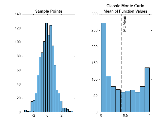
Plot the sample, function values, and calculated mean.

tiledlayout(1,2)
nexttile
h1 = histogram(sampleData);
title("Sample Points")
nexttile
h2 = histogram(funcValues);
hold on
xline(MCMean,'--','MCMean');
hold off
title("Classic Monte Carlo","Mean of Function Values")

QMC Methodology

First, define some parameters for the quantum simulation. Define the number of qubits for the probability distribution register as 5, and the number of qubits for the estimation register as 6. Then, discretize the probability distribution and function over a grid and compute the discrete mean of the function.

m = 5;  % Number of probability qubits
n = 6;  % Number of estimation qubits
M = 2^m;
N = 2^n;
probQubits = 1:m; 

x_max = pi;
x = linspace(-x_max,x_max,M)';
p = normpdf(x);
p = p./sum(p);

DiscreteMean = sum(func(x).*p)

DiscreteMean = 0.4326

The QMC methodology covered in [1] consists of the steps

Load the probability distribution onto a quantum register of m qubits.
Encode the value of the random variable onto a value qubit.
Use amplitude estimation, with a register of n qubits, to estimate the probability of the value qubit being in the state $|1anglebracketright$ .

While there are other approaches for amplitude estimation (such as iterative amplitude estimation), this example uses quantum phase estimation.

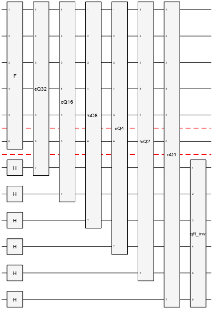
The circuit diagram below summarizes the approach. The F block loads the probability distribution and encodes the random variable onto a value qubit. The Q blocks and the inverse Quantum Fourier Transform (QFT) are used for quantum phase estimation.

Image of quantum circuit for QMC

1. Load Probability Distribution

Load the probability distribution onto m qubits. While [1] uses a quantum variational circuit to approximate the probability distribution, this example loads the probabilities directly onto the circuit. This requires the use of some custom gate functions:

%%%%%%%%%%%%%%%%%%%%%%%%%%%%%%%%%%%%%%%%%%%%%%%%%%%%%%%%%%%%%%%%%%%%%%
function cg = initStateToProbabilities(p)
% This function initializes their state so that the probabilities of
% measuring each state match vector p. Applied to a set of qubits all in
% state |0>.

L = log2(numel(p));
assert(numel(p) == 2^L);

theta = cell(1,L);

for lvl=1:L
    pp = reshape(p,2^(L-lvl),[]);
    pp = sum(pp,1);
    pp = reshape(pp,2,[]);
    theta{lvl} = 2*acos(sqrt(pp(1,:) ./ sum(pp,1)));
end

gates = ryGate(1,theta{1});

for lvl=2:log2(length(p))
    gates = [gates; ucrGate(1:lvl-1,lvl,theta{lvl}(:),'y')]; %#ok<AGROW>
end
cg = compositeGate(gates,1:L,Name="initP");
end
%%%%%%%%%%%%%%%%%%%%%%%%%%%%%%%%%%%%%%%%%%%%%%%%%%%%%%%%%%%%%%%%%%%%%%
function cg = ucrGate(controlQubits,targetQubit,theta,axis)
% Returns a CompositeGate implementing a uniformly-controlled rotation 
% about the specified axis on a target qubit.
%
% A rotation is applied for each classical state of controlQubits, so theta
% must be a vector of length 2^length(controlQubits).
%
% Reference:
% [1] Möttönen, M., J.J. Vartiainen, V. Bergholm, & M.M. Salomaa. "Quantum
%     Circuits for General Multi-qubit Gates." Physical Review Letters 93,
%     130502 (2004). https://arxiv.org/abs/quant-ph/0404089

arguments
    controlQubits
    targetQubit
    theta double {mustBeVector}
    axis {mustBeTextScalar}
end

Nc = length(controlQubits);

% Input checks
assert(log2(length(theta))==Nc)
assert(iscolumn(theta))
assert(ismember(axis,["x","y","z"]))

% Apply Walsh-Hadamard transformation 
Mk = hadamard(2^Nc);
invMk = 2^(-Nc) * Mk';
angles = invMk*theta;

% Permute the angles according to the Gray code
code = buildGrayCode(Nc);
perm = bin2dec(code)+1;
permAngles = angles(perm);

% Determine positions of control qubits from Gray code
isCtrl = code(1:2^Nc-1,:)~=code(2:2^Nc,:);
[ctrls,~] = find(isCtrl');
% Known by construction
ctrls(end+1) = 1;

% Construct local circuit with the control qubits at the top, followed by
% the target qubit
trgt = Nc+1;
if axis=="y"
    rotGates = ryGate(trgt,permAngles);
    entgGates = cxGate(ctrls,trgt);
elseif axis=="z"
    rotGates = rzGate(trgt,permAngles);
    entgGates = cxGate(ctrls,trgt);
elseif axis=="x"
    rotGates = rxGate(trgt,permAngles);
    entgGates = czGate(ctrls,trgt); 
end

% Merge rotation and entangling gates to build the circuit
gates = reshape([rotGates'; entgGates'],[],1);

% Map the local circuit to the desired qubits
cg = compositeGate(gates,[controlQubits(:); targetQubit],Name="ucr"+axis);

function code = buildGrayCode(n)
% 2^n-by-n char array defining the n-bit Gray Code.
%
% The rows of code contain every possible bit-string of length n arranged
% so that two neighboring rows only differ by one bit.

code = repmat('0',2^n,n); % Preallocate

code(:,1) = repelem('01',2^(n-1));

for ii=2:n
    block = repelem('0110',2^(n-ii));
    code(:,ii) = repmat(block,1,2^(ii-2));
end
end
end

Call initStateToProbabilities to initialize the circuit.

A = initStateToProbabilities(p);
A.Name = 'Ainit';

Simulate the register to verify that the probability distribution loaded correctly.

circ = quantumCircuit(A);
state = simulate(circ);
figure
histogram(state,probQubits)
title("Simulated Probabilities")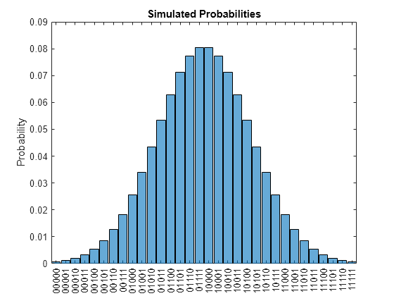

2. Encode Random Variable

Encode the discretized random variable function onto a value qubit.

valueQubit = m + 1;                        % Value qubit index
estQubits = (valueQubit + 1):(n + m + 1);  % Estimation qubits index

anglesR = 2*asin(sqrt(func(x)));

R = inv(ucrGate(probQubits,valueQubit,anglesR,"y"));
R.Name = "R";

Compute the probability of the value qubit being in the state $|1anglebracketright$ . The purpose of the F circuit is to evaluate the expected value of the random variable function.

F = compositeGate([A; R],[probQubits valueQubit],Name="F");
sF = simulate(quantumCircuit(F));
probability(sF,valueQubit,"1")

ans = 0.4326

3. Quantum Phase Estimation

Estimate the value of the value qubit using quantum phase estimation.

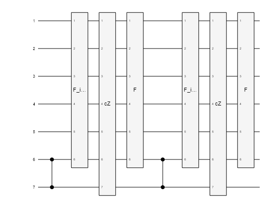
The controlled-Q block in the circuit diagram is implemented with several composite gates as outlined in [1]. Create a composite gate to represent this circuit element and plot the circuit to see the gates it contains.

controlQubit = valueQubit+1; % Re-mapped to estQubits in the loop below

cV = czGate(controlQubit,valueQubit); % For simplicity, do not wrap in a named CompositeGate

cZgates = [xGate([probQubits valueQubit])
          hGate(probQubits(1))
          mcxGate([probQubits(2:end) valueQubit controlQubit],probQubits(1),[])
          hGate(probQubits(1))
          xGate([probQubits valueQubit])];

cZ = compositeGate(cZgates,1:controlQubit,Name="cZ");

% Put the gates together to form controlled Q:

cQ = compositeGate([cV; inv(F); cZ; F; cV; inv(F); cZ; F],...
                   [probQubits valueQubit controlQubit],Name='cQ');

QPE = [];
for ii=1:n
    % Repeat the cQ gate as needed and map to the current control qubit:
    cQrep = compositeGate(repmat(cQ,2^(n-ii),1),...
                          [probQubits valueQubit estQubits(ii)],...
                          Name="cQ"+2^(n-ii));

    QPE = [QPE; cQrep]; %#ok<AGROW>
end

plot(cQ)

Simulate Final Circuit

Assemble the final circuit using the various component circuits, and plot the result. Specify the QubitBlocks name-value argument to display the two registers and the single value qubit.

circ = quantumCircuit([F;
                       hGate(estQubits); 
                       QPE; 
                       inv(qftGate(estQubits))]);
plot(circ,"QubitBlocks",[m 1 n])

Simulate the circuit.

state = simulate(circ);

Compare Results

In terms of the phase $θ$ , the analytical mean is given by

$μ = \frac{1 - \cos (π θ)}{2}$

Solve for $θ$ using the analytic value for $μ$ .

AnalyticPhase = acos(-2*AnalyticMean + 1)/pi

AnalyticPhase = 0.4568

Compare the analytic phase with the quantum phase estimation.

[states,probabilities] = querystates(state,estQubits);
plot(bin2dec(states)/N,probabilities)
xlim([.35 .65])
xline(AnalyticPhase,'--',"AnalyticPhase")
xlabel("\theta")
ylabel("Probability")
title("Phase Estimation with QMC")

The estimated phase is the first maximum in amplitude. Use the estimated phase to compute the mean value of the function, and compare the quantum value against the analytic value, classic Monte Carlo value, and discrete value.

y_ind = find(abs(probabilities - max(probabilities)) < 1e3*eps,1);
phase_estimated = bin2dec(states(y_ind))/N;
QMCMean = (1 - cos(pi * phase_estimated)) / 2;

ResultTable = table(AnalyticMean,MCMean,DiscreteMean,QMCMean)

ResultTable=1×4 table
    AnalyticMean    MCMean     DiscreteMean    QMCMean
    ____________    _______    ____________    _______

      0.43233       0.42103      0.43264       0.42663

References

[1] Priazhkina, S., V. Skavysh, D. Guala, & T. Bromley. "Quantum Monte Carlo for Economics: Stress Testing and Macroeconomic Deep Learning." Bank of Canada working paper (2022). https://www.bankofcanada.ca/wp-content/uploads/2022/06/swp2022-29.pdf

[2] Brassard, G., P. Hoyer, M. Mosca, & A. Tapp. "Quantum Amplitude Amplification and Estimation." Contemporary Mathematics 305 (2002): 53-74. https://arxiv.org/pdf/quant-ph/0005055.pdf

[3] Rebentrost, P., B. Gupt, & T. R. Bromley. "Quantum Computational Finance: Monte Carlo Pricing of Financial Derivatives." Physical Review A, 98(2), 022321 (2018). https://arxiv.org/pdf/1805.00109.pdf

[4] Stamatopoulos, N., D. J. Egger, Y. Sun, C. Zoufal, R. Iten, N. Shen, & S. Woerner. "Option Pricing Using Quantum Computers." Quantum 4, 291 (2020). https://arxiv.org/pdf/1905.02666.pdf

[5] Woerner, S., & D. J. Egger. "Quantum Risk Analysis." npj Quantum Information 5(1), 15 (2019). https://arxiv.org/pdf/1806.06893.pdf

Quantum Monte Carlo (QMC) Simulation

Problem Formulation

Classic Monte Carlo

QMC Methodology

1. Load Probability Distribution

2. Encode Random Variable

3. Quantum Phase Estimation

Simulate Final Circuit

Compare Results

References

See Also

Related Topics

Quantum Monte Carlo (QMC) Simulation

Problem Formulation

Classic Monte Carlo

QMC Methodology

1. Load Probability Distribution

2. Encode Random Variable

3. Quantum Phase Estimation

Simulate Final Circuit

Compare Results

References

See Also

Related Topics

WeChat