Solve XOR Problem Using Quantum Neural Network (QNN)

This example uses:

This example shows how to solve the XOR problem using a trained quantum neural network (QNN). You use the network to classify the classical data of 2-D coordinates. A QNN is a machine learning model that combines quantum computing layers and classical layers. This example shows how to train such a hybrid network for a classification problem that is nonlinearly separable, such as the exclusive-OR (XOR) problem.

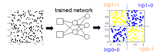
Classification of 2-D data points in the XOR problem using a trained network

In the XOR problem, two-dimensional (2-D) data points are classified based on the region of their x- and y-coordinates using a mapping function that resembles the XOR function. If the x- and y-coordinates are both in region 0 or 1, then the data are classified into class "0". Otherwise, the data are classified into class "1". In this problem, a single linear decision boundary cannot solve the classification problem. Instead, nonlinear decision boundaries are required to classify the data.

This example shows a proof-of-concept idea about how to train a QNN using a local simulation. For more general frameworks using a hybrid quantum-classical model to classify quantum and classical data, see references [1] and [2]. The QNN in this example consists of four layers:

A feature input layer for the XOR problem.
A parameterized quantum circuit (PQC) as the ansatz circuit. This circuit prepares the states of qubits according to the coordinates of the input data with learnable parameters. The circuit then measures the probability distributions of the quantum states along the z-axis and passes them to the next layers.
A fully connected layer that applies a linear transformation to the quantum circuit measurements through a weight matrix and a bias vector.
A two-output softmax layer, which outputs probabilities for the data classification.

Quantum neural network with quantum computing and classical layers

Finally, the network computes a loss function based on the categorical cross-entropy between the predictions and the labels. The network then propagates the gradients of the loss with respect to the learnable parameters through the layers to train the QNN using the stochastic gradient descent with momentum (SGDM) optimization.

Generate Training Data

The generateData function creates a sample of data points for the XOR problem. This function classifies data into two groups: "Blue" and "Yellow". If the coordinates of the data points satisfy $x > 1$ and $y > 0.5$ , or $x < 1$ and $y < 0.5$ , then this function classifies the data points as "Blue". Otherwise, if the coordinates of the data points satisfy $x > 1$ and $y < 0.5$ , or $x < 1$ and $y > 0.5$ , then this function classifies the data points as "Yellow".

function [X,Y] = generateData(numSamples)
    X = zeros(numSamples,2);
    labels = strings(numSamples,1);
    for i = 1:numSamples
        x1 = 2*rand;
        x2 = rand;
        X(i,:) = [x1 x2];
        if (x1 > 1 && x2 > 0.5) || (x1 < 1 && x2 < 0.5)    
            labels(i) = "Blue";
        else
            labels(i) = "Yellow";
        end
    end
    Y = categorical(labels);
end

Generate training data with 200 data points using the generateData function. The network classifies the data into the "Blue" and "Yellow" classes.

numSamples = 200;
[X,Y] = generateData(numSamples);
classNames = ["Blue", "Yellow"];

The input for each data point has the form of 2-D coordinates. Specify the number of classes in the training data.

inputSize = size(X,2);
numClasses = numel(classNames);

Create Parameterized Quantum Computing layer

Define a custom layer for the quantum circuit. For more information about creating a custom deep learning layer in MATLAB®, see Define Custom Deep Learning Layer with Learnable Parameters (Deep Learning Toolbox).

Forward Pass

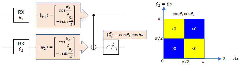
The quantum circuit consists of two qubits that are initially in the $|0anglebracketright$ state. Construct the quantum circuit by applying an RX gate with the rotation angle $θ_{1}$ to the first qubit and an RX gate with the rotation angle $θ_{2}$ to the second qubit, followed by a controlled NOT gate to the first qubit as the control and the second qubit as the target. These gates prepare the states of the qubits according to the coordinates of the input data by introducing two adjustable learnable parameters A and B in the rotation angles. These parameters are the scaling factors for the rotation angles of each qubit, which scale the x- and y-coordinates of the XOR problem to $θ_{1} = Ax$ and $θ_{2} = By$ . You then perform a measurement on the second qubit in the Z basis. The quantity of interest is the magnetization of the second qubit, which is the difference in counts of this qubit being in the $|0anglebracketright$ state and the $|1anglebracketright$ state. For this quantum circuit, the measured quantity $⟨ \hat{Z} ⟩$ has a predicted form of $\cos θ_{1} \cos θ_{2}$ based on the states of the qubits. You then use the condition $⟨ \hat{Z} ⟩ = 0$ to determine the classification boundaries of the XOR problem. In this conceptual example, you use local simulation to determine the probabilities of measuring the qubit in these states instead of real counts on quantum hardware.

Forward pass by the quantum gates in the parameterized quantum circuit

Backpropagation

To train the network, the derivative of the loss function through the quantum computing layer needs to be backpropagated. Backpropagation requires the computation of the gradients of $⟨ \hat{Z} ⟩$ with respect to the learnable parameters. To find these gradients, use the parameter-shift rules that are valid at the operator level, as described in [3] and [4]. For this quantum circuit, these equations give the gradients of $⟨ \hat{Z} ⟩$ with respect to the learnable parameters A and B.

$\begin{array}{l} \frac{\partial}{\partial A} ⟨ \hat{Z} (A, B) ⟩ = x \frac{⟨ \hat{Z} (A + s, B) ⟩ - ⟨ \hat{Z} (A - s, B) ⟩}{2 \sin (sx)} \\ \frac{\partial}{\partial B} ⟨ \hat{Z} (A, B) ⟩ = y \frac{⟨ \hat{Z} (A, B + s) ⟩ - ⟨ \hat{Z} (A, B - s) ⟩}{2 \sin (sy)} \end{array}$

As in [3], the gradients of the expectation values are exact for any choice of s as long as s is not an integer multiple of $π$ . This example chooses $s = \frac{π}{4}$ .

Define Custom Layer

To create a custom layer for the quantum circuit, create the PQCLayer class with this definition:

In the properties block, define the learnable parameters A and B.
Specify the layer constructor function as PQCLayer. In the constructor, specify the layer name, the layer description, and the initial values of the learnable parameters.
Specify the predict layer, which computes the $⟨ \hat{Z} ⟩$ measurement at prediction time.
Specify the backward layer, which backpropagates the derivative of the loss function through the layer. You do not need the gradients of $⟨ \hat{Z} ⟩$ with respect to the x- and y-coordinates because you do not use the gradients of the loss function with respect to x and y during training.
Specify a computeZ function that defines the quantum circuit and computes the $⟨ \hat{Z} ⟩$ measurement. Create the quantum circuit with two qubits by using quantumCircuit. Add the two RX gates with the rotation angles $θ_{1} = Ax$ and $θ_{2} = By$ by using rxGate and the CNOT gate by using cxGate. Locally simulate the final state of the quantum circuit by using simulate. Compute the predicted $⟨ \hat{Z} ⟩$ measurement on the second qubit by using the probability function to find the difference in counts of this qubit being in the $|0anglebracketright$ state and the $|1anglebracketright$ state.

Save the PQCLayer class definition in a separate file on the path.

classdef PQCLayer < nnet.layer.Layer
    % Custom PQC layer example.

    properties (Learnable)
        % Define layer learnable parameters.
        A
        B
    end

    methods
        function layer = PQCLayer
            % Set layer name.
            layer.Name = "PQC";

            % Set layer description.
            layer.Description = "Layer containing a parameterized " + ...
                "quantum circuit (PQC)";

            % Initialize learnable parameter.
            layer.A = 1;
            layer.B = 2;
        end

        function Z = predict(layer,X)
            % Z = predict(layer,X) forwards the input data X through the
            % layer and outputs the result Z at prediction time.
            Z = computeZ(X,layer.A,layer.B);
        end

        function [dLdX,dLdA,dLdB] = backward(layer,X,Z,dLdZ,memory)
            % Backpropagate the derivative of the loss
            % function through the layer.
            %
            % Inputs:
            %     layer   - Layer though which data backpropagates
            %     X       - Layer input data
            %     Z       - Layer output data
            %     dLdZ    - Derivative of loss with respect to layer
            %               output
            %     memory  - Memory value from forward function
            % Outputs:
            %     dLdX   - Derivative of loss with respect to layer input
            %     dLdA   - Derivative of loss with respect to learnable
            %              parameter A
            %     dLdB   - Derivative of loss with respect to learnable
            %              parameter B

            s = pi/4;
            ZPlus = computeZ(X,layer.A + s,layer.B);
            ZMinus = computeZ(X,layer.A - s,layer.B);
            dZdA = X(1,:).*((ZPlus - ZMinus)./(2*sin(X(1,:).*s)));
            dLdA = sum(dLdZ.*dZdA,"all");

            ZPlus = computeZ(X,layer.A,layer.B + s);
            ZMinus = computeZ(X,layer.A,layer.B - s);
            dZdB = X(2,:).*(((ZPlus - ZMinus)./(2*sin(X(2,:).*s))));
            dLdB = sum(dLdZ.*dZdB,"all");

            % Set the gradients with respect to x and y to zero
            % because the QNN does not use them during training.
            dLdX = zeros(size(X),"like",X);
        end
    end
end

function Z = computeZ(X, A, B)
    numSamples = size(X,2);
    x1 = X(1,:);
    x2 = X(2,:);
    Z = zeros(1,numSamples,"like",X);
    for i = 1:numSamples
        circ = quantumCircuit(2);
        circ.Gates = [rxGate(1,x1(i)*A); rxGate(2,x2(i)*B); cxGate(1,2)];
        s = simulate(circ);
        Z(i) = probability(s,2,"0") - probability(s,2,"1");
    end
end

Define Network Architecture

Define the layers in the QNN that you train to solve the XOR problem.

Create a feature input layer with observations consisting of two features. These features correspond to the coordinates of the XOR problem.
Specify a quantum computing layer using the PQCLayer class.
For classification, specify a fully connected layer with a size equal to the number of classes.
Map the output to probabilities by including a two-output softmax layer.
Create an output classification layer that computes the cross-entropy loss between the true labels and the probabilities output of the softmax layer.

layers = [featureInputLayer(inputSize,Normalization="none")
          PQCLayer
          fullyConnectedLayer(numClasses)
          softmaxLayer
          classificationLayer];

Specify Training Options

Configure the SGDM optimization with a mini-batch size of 20 at each iteration, a learning rate of 0.1, and a momentum of 0.9. Use the CPU to train the network. Turn on the training progress plot and suppress the training progress indicator in the Command Window.

options = trainingOptions("sgdm", ...
    MiniBatchSize=20, ...
    InitialLearnRate=0.1, ...
    Momentum=0.9, ...
    ExecutionEnvironment="cpu", ...
    Plots="training-progress", ...
    Verbose=false);

Train Network

Train the QNN. The result shows an excellent accuracy above 90% for classifying the XOR problem.

net = trainNetwork(X,Y,layers,options)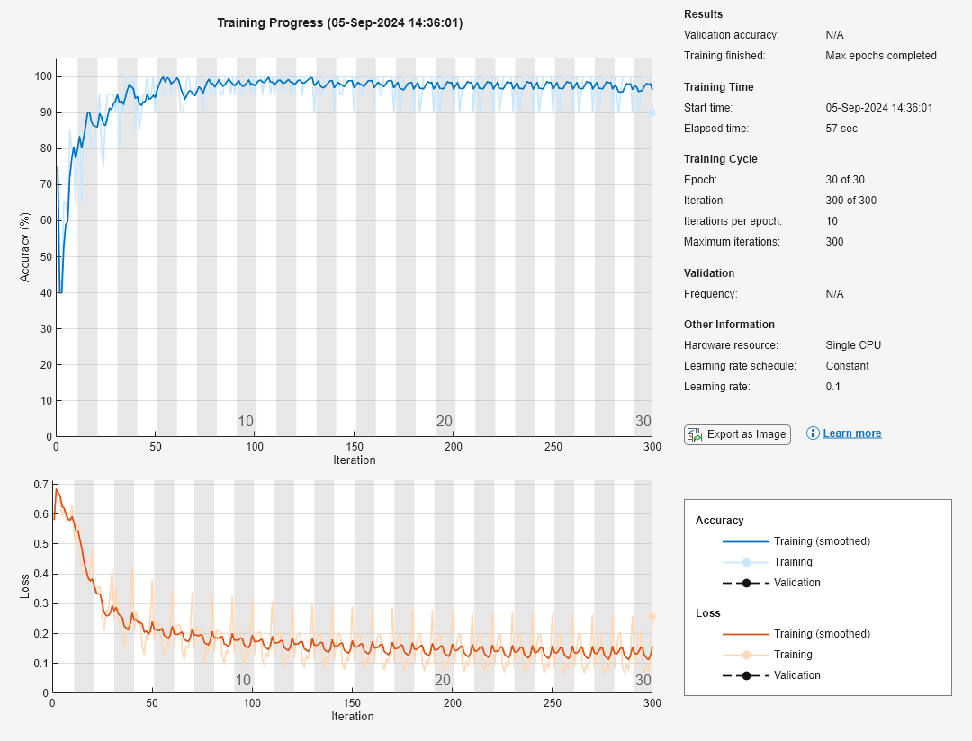

net = 
  SeriesNetwork with properties:

         Layers: [5x1 nnet.cnn.layer.Layer]
     InputNames: {'input'}
    OutputNames: {'classoutput'}

Test Network

Test the classification accuracy of the network by comparing the predictions on the test data with the true labels.

Generate new test data not used during training.

[XTest,trueLabels] = generateData(numSamples);

Find the predicted classification for the test data.

predictedLabels = classify(net,XTest);

Plot the predicted classification for the test data.

gscatter(XTest(:,1),XTest(:,2),predictedLabels,"by")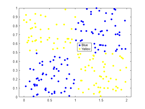

Visualize the accuracy of the predictions in a confusion chart. Large values on the diagonal indicate accurate predictions for the corresponding class. Large values on the off-diagonal indicate strong confusion between the corresponding classes. Here, the confusion chart shows very small errors in classifying the test data.

confusionchart(trueLabels,predictedLabels)

References

[1] Broughton, Michael, Guillaume Verdon, Trevor McCourt, Antonio J. Martinez, Jae Hyeon Yoo, Sergei V. Isakov, Philip Massey, et al. "TensorFlow Quantum: A Software Framework for Quantum Machine Leanring." Preprint, submitted August 26, 2021. https://doi.org/10.48550/arXiv.2003.02989.

[2] Farhi, Edward, and Hartmut Neven. "Classification with Quantum Neural Networks on Near Term Processors." Preprint, submitted August 30, 2018. https://doi.org/10.48550/arXiv.1802.06002.

[3] Mari, Andrea, Thomas R. Bromley, and Nathan Killoran. “Estimating the Gradient and Higher-Order Derivatives on Quantum Hardware.” Physical Review A 103, no. 1 (January 11, 2021): 012405. https://doi.org/10.1103/PhysRevA.103.012405.

[4] Wierichs, David, Josh Izaac, Cody Wang, and Cedric Yen-Yu Lin. “General Parameter-Shift Rules for Quantum Gradients.” Quantum 6 (March 30, 2022): 677. https://doi.org/10.22331/q-2022-03-30-677.