Control Robot Manipulator Using C/GMRES Solver

Open Live Script

This example shows how to design a multistage nonlinear model predictive controller that uses the C/GMRES solver to control a robot manipulator.

Background

Nonlinear receding horizon control (RHC), also known as nonlinear model predictive control (MPC), is a strategy to control dynamic systems. It consists in calculating the optimal sequence of control actions over a finite time horizon while implementing only the first action. The control sequence is recalculated as time progresses, considering updated measurements and a shifted time horizon.

To guide the optimization process, RHC incorporates the concepts of stage cost and terminal cost, where:

Stage cost: The stage cost represents the cost associated with each stage (the time step) of the control problem. It quantifies the immediate cost (also known as penalty) incurred at each step. In this example, the stage cost is defined using a standard quadratic cost function that penalizes the deviation of the state vector $x$ from the desired state $x_{f}$ at each time point within the horizon, $k$ , and the control effort, $u$ , required to achieve the desired state.

$L (x (τ), u (τ), pv) = {(x - x_{f})}^{T} Q (x - x_{f}) + u^{T} R u$

Terminal cost: This term represents a cost (also sometimes called penalty) associated with the final state of the system. The terminal penalty penalizes the deviation of the state at the end of the horizon $x_{p + 1}$ , from the desired state $x_{f}$ , where $p + 1$ is the final stage, which corresponds to the end of the prediction horizon, $t + T$ .

$φ (x (t + T), pv) = \frac{1}{2} {(x (t + T) - x_{f})}^{T} S_{f} (x (t + T) - x_{f})$

Here, the matrices $Q$ and $R$ determine the weight of the state deviation from the desired state, and the control effort, respectively. The matrix $S_{f}$ determines the weight for the terminal penalty, and $pv$ is the stage parameter vector.

The overall performance index for the receding horizon control problem is given by:

$J = φ (x (t + T), pv) + \frac{1}{2} \int_{t}^{t + T} L (x (τ), u (τ), pv) d τ$

The formulation of RHC allows for the independent specification of stage costs for each time step, making it suitable for multistage nonlinear MPC controllers.

Nonlinear Model

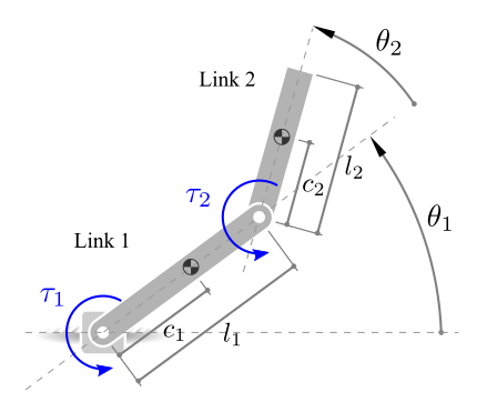
This figure gives the schematics of the two-link planar robot.

The configuration of the robot is determined by the joint angles $θ_{1}$ and $θ_{2}$ , along with the torques $τ_{1}$ and $τ_{2}$ applied at the joints to control the position of the robot's tip.

The state vector is defined as:

$x (t) = [\begin{array}{c} q \\ \dot{q} \end{array}]$ , where $q = [\begin{array}{c} θ_{1} \\ θ_{2} \end{array}]$ .

The dynamics for a two-link robot manipulator can be expressed as follows [1]:

$H (q) \ddot{q} + C (q, \dot{q}) \dot{q} + G (q) = τ$ .

Here, $q$ , $\dot{q}$ , and $\ddot{q}$ are 2-by-1 vectors that represent the joint angles, velocities, and accelerations. The control input vector is the torque $τ$ . The remaining terms correspond to manipulator inertia matrix, $H (q)$ , Coriolis matrix, $C (q, \dot{q})$ , and gravity vector, $G (q)$ .

This robot dynamics is implemented in twolinkStateFcn.m. This file is a MATLAB® function that takes as inputs the state vector, $x$ , the control input vector, $u$ , and a vector of model parameters, $pvstate$ . The function's output is the vector of the state derivatives with respect to time.

The physical parameters of the robot are defined in the following table:

% Two-Link Robot Physical Parameter Values.
Value = [0.3; 0.15; 0.2; 
         6.0e-3; 0.3; 0.257; 
         0.7; 5.1e-2; 9.81];

Units = ["m"; "m"; "kg"; 
         "kg*m^2"; "m"; "m"; 
         "kg"; "kg*m^2"; "m/s^2"];

Param = [ ...
    "Length, L1", "Center of mass, s1", "Mass, m1", ...
    "Moment of Inertia, J1", "Length, L2", ...
    "Center of mass, s2", "Mass, m2", ...
    "Moment of Inertia, J2", "Gravity, g"];

% Convert arrays to table
ParamTable = array2table(Value, "RowNames", Param);
UnitsTable = table(categorical(Units), ...
                   VariableNames = "Units");
% Display parameter values.

disp([ParamTable UnitsTable])

                             Value    Units 
                             _____    ______

    Length, L1                 0.3    m     
    Center of mass, s1        0.15    m     
    Mass, m1                   0.2    kg    
    Moment of Inertia, J1    0.006    kg*m^2
    Length, L2                 0.3    m     
    Center of mass, s2       0.257    m     
    Mass, m2                   0.7    kg    
    Moment of Inertia, J2    0.051    kg*m^2
    Gravity, g                9.81    m/s^2

Define model parameter vector:

pvstate = ParamTable.Value;

Define Objective Cost Function

The control strategy involves optimizing the performance index, $J$ , over a finite time horizon and is given by:

$J = \frac{1}{2} {(x (t + T) - x_{f})}^{T} S_{f} (x (t + T) - x_{f}) + \frac{1}{2} \int_{τ}^{τ + T} ({(x - x_{f})}^{T} Q (x - x_{f}) + u^{T} R u) d τ$

where:

$x_{f}$ represents the desired state.
$S_{f}$ , $Q$ , and $R$ are weight matrices that determine the importance of different terms in the performance index.

The $S_{f}$ , $Q$ , and $R$ values impact the control strategy and the trade-off between tracking the objective state and minimizing control effort.

For this example, define the weight matrices as a column vector and combine state parameter into the pvcost variable.

% Stage Parameters
Sf = [20; 10; 1e-3; 1e-3];  % Terminal Weight Matrix.
Q  = [30; 30; 1e-3; 1e-3];  % State Weight Matrix.
R  = [0.1; 0.1];            % Control Weighting Matrix.

Append the prediction horizon of the controller and desired state to the stage parameter. For this example, the prediction horizon uses 50 steps.

p  = 50;                    % Prediction Horizon.
xf = [1; 1; 0; 0];          % Terminal State.

% Combine stage parameters into a column array.
pvcost = [xf; Sf; Q; R; p];

The objective cost function is implemented in the MATLAB function twolinkCostFcn.m.

type("twolinkCostFcn.m")

function L = twolinkCostFcn(stage, x, u, pvcost)
% twolinkCostFcn
%   L = twolinkCostFcn(stage, x, u, pvcost)
%   
%   This function computes the objective cost for the two-link robot
%   manipulator example.
%
%   Inputs:
%       - stage     Current stage of the Multistage MPC problem
%       - x         Current state vector
%       - u         Control action vector at the previous interval
%       - pvcost    Vector containing various stage parameters
%
%   Output:
%       - L:        Cost value calculated by the cost function.

% Copyright 2023 The MathWorks, Inc.

% Extract Desired State
xf = pvcost(1:4);

% Extract and Initialize Wiegthing Matrices
Sf = diag(pvcost(5:8));                 % Terminal Weight Matrix
Q  = diag(pvcost(9:12));                % State Weight Matrix
R  = diag(pvcost(12+(1:length(u))));    % Control Weight Matrix
p  = pvcost(15);                        % Prediction Horizon

if stage == p + 1
    % Calculate cost for the terminal stage
    L = 0.5*(x - xf).'*Sf*(x - xf);
else
    % Calculate cost for intermediate stages
    L = 0.5*(x - xf).'*Q*(x - xf) + 0.5*u.'*R*u;
end
end

Robot Environment

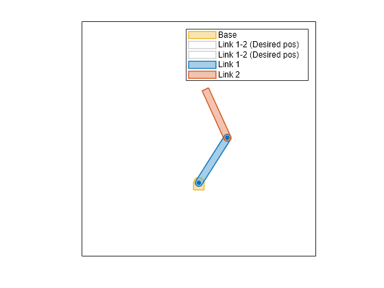
The robot environment contains a two-link robot. For this example, the objective is to have the robot follow a given reference trajectory, starting at zero angular position and velocity.

% Define Initial State.
x0 = [0; 0; 0; 0];

% Initialize Two Link Robot plot.
figure("Color", "w")
hPlot = helperRobotEnvironment( ...
    Length1 = pvstate(1), ...
    Length2 = pvstate(5));

% Set Initial angular position and desired state. 
hPlot.Theta1 = x0(1);
hPlot.Theta2 = x0(2);
hPlot.xf = xf;

Figure contains an object of type helperrobotenvironment.

The animation plot is initialized to display both the initial position of the manipulator robot and the target position.

Design Nonlinear MPC Controller

Create a nonlinear multistage MPC object with four states and two inputs.

nx  = 4;
nmv = 2;
msobj = nlmpcMultistage(p,nx,nmv);

In this example, the target prediction time is 0.1 seconds. Therefore, for a prediction horizon of 50 steps specify a sample time of 0.002 seconds.

Ts = 2e-3;
msobj.Ts = Ts;

Specify the prediction model state and Jacobian functions using the robot dynamics functions.

msobj.Model.StateFcn = "twolinkStateFcn";
msobj.Model.StateJacFcn = "twolinkStateJacFcn";
msobj.Model.ParameterLength = length(pvstate);

Specify this cost function using a named function. For more information on specifying cost functions, see Specify Cost Function for Nonlinear MPC.

% Setting cost function for each control interval.
for k = 1:p+1
    msobj.Stages(k).CostFcn = "twolinkCostFcn";
    msobj.Stages(k).CostJacFcn = "twolinkCostJacFcn";
    msobj.Stages(k).ParameterLength = length(pvcost);
end

Specify hard bounds on the two joint motors.

msobj.ManipulatedVariables(1).Min = -10;
msobj.ManipulatedVariables(1).Max =  10;
msobj.ManipulatedVariables(2).Min = -10;
msobj.ManipulatedVariables(2).Max =  10;

The state and stage functions require state and stage parameters. Use getSimulationData to initialize data structure. For more information on simulation data structure for multistage MPC, see getSimulationData.

simdata = getSimulationData(msobj);
simdata.StateFcnParameter = pvstate;
simdata.StageParameter = repmat(pvcost, p+1, 1);

Setting the Optimization Solver

The optimization solver finds the optimal control inputs that minimize a given cost function while satisfying constraints. Configuring the solver options correctly can improve the efficiency and accuracy of the optimization process.

Specify the optimization solver using the Solver property of the multistage MPC object. Choose either fmincon or cgmres based on your requirements.

For this example, set the multistage MPC object to use the cgmres solver [2].

msobj.Optimization.Solver = "cgmres";

It is recommended to tune the stabilization parameter according to the prediction model sample time to further optimize solver performance. Adjust the StabilizationParameter property of the multistage MPC object by assigning an appropriate value between $\frac{1}{T_{s}}$ and $\frac{2}{T_{s}}$ . Smaller values results in lower step sizes for the solver.

% Adjust the Stabilization Parameter 
% based on the prediction model sample time.
msobj.Optimization.SolverOptions.StabilizationParameter = 1/msobj.Ts;

% Set the solver parameters.
msobj.Optimization.SolverOptions.MaxIterations = 10;
msobj.Optimization.SolverOptions.Restart = 3;
msobj.Optimization.SolverOptions.BarrierParameter = 1e-3;
msobj.Optimization.SolverOptions.TerminationTolerance = 1e-6;

For more information on configuring the cgmres solver, see Configure C/GMRES Solver Options and the Optimization property of nlmpcMultistage.

Code Generation in MATLAB

To speed up computation time during simulation, use getCodeGenerationData and buildMEX to generate code for the Multistage MPC object with the specified properties.

Generate data structures using getCodeGenerationData.

u0 = zeros(nmv,1);
[coredata, onlinedata] = getCodeGenerationData( ...
    msobj, x0, u0, ...
    StateFcnParameter=pvstate, ...
    StageParameter=repmat(pvcost, p+1, 1));

Generate a MEX function called nlmpcControllerMEX.

buildMEX(msobj, "nlmpcControllerMEX", coredata, onlinedata);

Generating MEX function "nlmpcControllerMEX" from your "nlmpcMultistage" object to speed up simulation.
Code generation successful.

MEX function "nlmpcControllerMEX" successfully generated.

It is best practice to compare the optimization results from both the standard nlmpcmove and nlmpcmoveCodeGeneration function. Since optimization results might vary for distinct initial guess, use the same run-time data structure for comparison of the optimal solution for Multistage MPC.

Update the onlinedata structure with the state and stage parameters, and use the InitialGuess generated using nlmpcmove.

% Update onlinedata structure with state and stage parameters.
onlinedata.StateFcnParameter = simdata.StateFcnParameter;
onlinedata.StageParameter = simdata.StageParameter;
simdata.InitialGuess = onlinedata.InitialGuess;

Run and compare the optimization results using the same initial guess.

[~, ~, info1] = nlmpcmove(msobj, x0, u0, onlinedata);
[~, ~, info2] = nlmpcmoveCodeGeneration(coredata, x0, u0, onlinedata); 
[~, ~, info3] = nlmpcControllerMEX(x0, u0, onlinedata);

Plot optimization results:

figure;
for ix = 1:nx
    subplot(3,2,ix); hold on; box on;
    plot(info1.Topt, info1.Xopt(:,ix), "-.");
    plot(info2.Topt, info2.Xopt(:,ix), "-x");
    plot(info3.Topt, info3.Xopt(:,ix), "-+");
    title(['State, x_' num2str(ix)]);
    xlabel("Time, s");
end

for imv = 1:nmv
    subplot(3,2,ix+imv); hold on; box on;
    plot(info1.Topt, info1.MVopt(:,imv), "-.");
    plot(info2.Topt, info2.MVopt(:,imv), "-x");
    plot(info3.Topt, info3.MVopt(:,imv), "-+");
    title(['Control, u_' num2str(imv)]);
    xlabel("Time, s");
end

legend("nlmpcmove", ...
    "nlmpcmoveCodeGeneration", ...
    "nlmpcControllerMEX")

The plot shows a comparison between three distinct computations of the control action, demonstrating their equivalence as their results closely align with each other.

Closed-Loop Simulation in MATLAB

Simulate the system for 2 seconds with a target trajectory to follow using the MEX Function.

% Simulation duration in seconds.
Duration = 2;

% Store states and control for plotting purposes.
xHistory1 = x0.';
uHistory1 = u0.';

% Initialize current state and control.
xk = xHistory1(1,:).';
uk = uHistory1(1,:).';

% Initialize the accumulated elapsed time 
% for computing the optimal control action calculation.
timerVal1 = 0;

% Simulation loop
for k = 1:(Duration/Ts)
    % Compute optimal control action using nlmpcmove.
    xk = xHistory1(k,:).';
    
    % Call the nlmpcControllerMEX function.
    tic
    [uk, onlinedata] = nlmpcControllerMEX(xk, uk, onlinedata);
    
    % Accumulate the elapsed time.
    timerVal1 = timerVal1 + toc;

    % Simulate Two-Link Robot for the next control interval.
    ODEFUN = @(t,xk) twolinkStateFcn(xk,uk,pvstate);
    [TOUT, XOUT] = ode45(ODEFUN, [0 Ts], xHistory1(k,:));

    % Log states and control.
    xHistory1(k+1,:) = XOUT(end,:);
    uHistory1(k+1,:) = uk;
    
    % Update two-link robot plot.
    hPlot.Theta1 = xHistory1(k+1,1);
    hPlot.Theta2 = xHistory1(k+1,2);
    drawnow limitrate

end

Figure contains an object of type helperrobotenvironment.

The animation shows that the manipulator robot successfully moves from the start position to desired target position using the MEX function.

% Plot the closed loop results.
figure;
helperPlotResults(xHistory1, uHistory1, Ts, xf, 'show')

$Figure contains 6 axes objects. Axes object 1 with title Joint Angle, theta indexOf 1 baseline, xlabel Time, s contains 2 objects of type line. These objects represent \theta_1, xf_1. Axes object 2 with title Joint Angle, theta indexOf 2 baseline, xlabel Time, s contains 2 objects of type line. These objects represent \theta_2, xf_2. Axes object 3 with title Joint Velocity, omega indexOf 1 baseline, xlabel Time, s contains 2 objects of type line. These objects represent \omega_1, xf_3. Axes object 4 with title Joint Velocity, omega indexOf 2 baseline, xlabel Time, s contains 2 objects of type line. These objects represent \omega_2, xf_4. Axes object 5 with title Torque, tau indexOf 1 baseline, xlabel Time, s contains an object of type line. This object represents \tau_1. Axes object 6 with title Torque, tau indexOf 2 baseline, xlabel Time, s contains an object of type line. This object represents \tau_2.$

The plot shows the joint angles, velocities, and torques of the manipulator robot. Additionally, it displays the desired states, indicating the successful attainment of the objective using the MEX function.

Closed-Loop Simulation Using Simulink

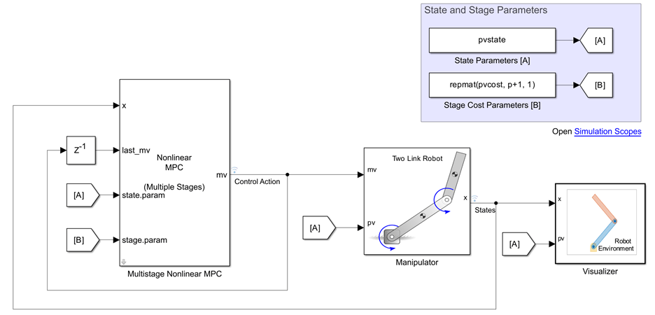
Open the Simulink® model.

mdl = 'twolinkMultistageNLMPC';
open_system(mdl)

Run the simulation with the MEX Function to speed up simulation.

tic
simHistory = sim(mdl, Duration);

Figure contains an object of type helperrobotenvironment.

The animation shows that the manipulator robot successfully moves from the start position to desired target position using Simulink.

timerVal2 = toc;

Plot all the simulation results.

% Use helperPlotResults function 
% to plot results stored in xHistory1,
% xHistory2, simHistory1, and simHistory2.
figure("Color", "w"); hold on;
helperPlotResults(simHistory)
helperPlotResults(xHistory1, uHistory1, Ts, [], "show")

$Figure contains 6 axes objects. Axes object 1 with title Joint Angle, theta indexOf 1 baseline, xlabel Time, s contains 2 objects of type line. These objects represent \theta_1. Axes object 2 with title Joint Angle, theta indexOf 2 baseline, xlabel Time, s contains 2 objects of type line. These objects represent \theta_2. Axes object 3 with title Joint Velocity, omega indexOf 1 baseline, xlabel Time, s contains 2 objects of type line. These objects represent \omega_1. Axes object 4 with title Joint Velocity, omega indexOf 2 baseline, xlabel Time, s contains 2 objects of type line. These objects represent \omega_2. Axes object 5 with title Torque, tau indexOf 1 baseline, xlabel Time, s contains 2 objects of type line. These objects represent \tau_1. Axes object 6 with title Torque, tau indexOf 2 baseline, xlabel Time, s contains 2 objects of type line. These objects represent \tau_2.$

Note that all employed simulations produce consistent state responses and control actions. Additionally, the elapsed time for each simulation is displayed in the following table:

timerVals = [timerVal1; timerVal2];

simNames  = {'MATLAB'; 'Simulink'};

SummaryTable = array2table(timerVals, ...
    "VariableNames", ...
    "Elapsed Time, sec");

SummaryTable.Properties.RowNames = simNames;
disp(SummaryTable)

                Elapsed Time, sec
                _________________

    MATLAB           1.9211      
    Simulink         13.647

References

[1] Hatanaka, Takeshi, Nikhil Chopra, Masayuki Fujita, and Mark W. Spong. Passivity-Based Control and Estimation in Networked Robotics. Communications and Control Engineering. Cham: Springer International Publishing, 2015. https://doi.org/10.1007/978-3-319-15171-7.

[2] Ohtsuka, T. “Continuation/GMRES Method for Fast Algorithm of Nonlinear Receding Horizon Control.” Proceedings of the 39th IEEE Conference on Decision and Control (Cat. No.00CH37187), vol. 1, 2000, pp. 766–71 vol.1. IEEE Xplore, https://doi.org/10.1109/CDC.2000.912861.

Control Robot Manipulator Using C/GMRES Solver

Background

Nonlinear Model

Define Objective Cost Function

Robot Environment

Design Nonlinear MPC Controller

Setting the Optimization Solver

Code Generation in MATLAB

Closed-Loop Simulation in MATLAB

Closed-Loop Simulation Using Simulink

References

See Also

Functions

Objects

Blocks

Related Examples

More About