Solve Fuel-Optimal Navigation Problem Using C/GMRES

Open Live Script

This example shows how to determine the optimal path for a boat to reach a destination by minimizing fuel expenditure, while being affected by a drift. You solve the problem using multistage nonlinear model predictive control (MPC) with the continuation/generalized minimum residual (C/GMRES) solver.

Traditionally, Zermelo's navigation problem deals with determining the minimum-time path for a boat moving from an initial location to a target destination across a watery expanse. The boat is capable of a maximum speed and is usually presented as a time-optimal control problem. The goal is to derive the best possible control to reach the destination B in the least possible time.

In this example, you address a specialized variant of the classic Zermelo's navigation problem, where the goal is to reach the destination using the least possible amount of fuel.

Problem Formulation

Consider a two-dimensional problem where a boat moves in the xy-plane. The state of the boat is given by its position $(x, y)$ and its velocity $v$ . The control inputs are the velocity $v$ and the direction $α$ of the boat. The drift is represented by a velocity vector $d (x, y)$ , which depends on the position of the boat.

The dynamics of the boat are represented by these differential equations:

$\dot{x} = v \cdot \cos (α) + d_{x} (x, y)$

$\dot{y} = v \cdot \sin (α) + d_{y} (x, y)$

where $d_{x}$ and $d_{y}$ are the components of the drift vector $d (x, y)$ .

For this example, the drift function is defined as $d (x, y) = [\begin{array}{c} 3 + 0.2 y \cdot (1 - y) \\ 0 \end{array}]$ .

For this example, the model and stage functions are encapsulated in the Navigation class (which is defined in the supporting file Navigation.m) as static methods.

Display the Navigation class.

type Navigation.m

classdef Navigation
    % Navigation class contains methods for state evolution, Jacobians,
    % cost functions, and inequality constraints for an MPC controller.

    % Copyright 2023 The MathWorks, Inc.

    methods (Static)
        function f = StateFcn(x,u,pvstate)
            % State evolution function without drift.
            % x: state vector
            % u: control input vector
            a = u(1); 
            V = u(2); 
            f = [V*cos(a); V*sin(a)];
        end

        function [fx,fu] = StateJacFcn(x,u,pvstate)
            % Jacobian of the state function without drift.
            % fx: Jacobian w.r.t. the state
            % fu: Jacobian w.r.t. the control input
            a = u(1); 
            V = u(2); 
            fx = [0, 0; 0, 0]; 
            fu = [-V*sin(a), cos(a); V*cos(a), sin(a)]; 
        end

        function f = StateFcnWithDrift(x,u,pvstate)
            % State evolution function with added drift.
            % The drift is a function of the state x(2).
            a = u(1); 
            V = u(2); 
            h = 3 + 0.2*x(2)*(1-x(2)); % Drift term as a function of x(2)
            f = [V*cos(a) + h; V*sin(a)];
        end

        function [fx,fu] = StateJacFcnWithDrift(x,u,pvstate)
            % Jacobian of the state function with drift.
            % fx: Jacobian w.r.t. the state
            % fu: Jacobian w.r.t. the control input
            a = u(1); 
            V = u(2); 
            hx = 1/5 - (2*x(2))/5; 
            fx = [0, hx; 0, 0]; 
            fu = [-V*sin(a), cos(a); V*cos(a), sin(a)]; 
        end

        function L = CostFcn(i,x,u,pvstage)
            % Cost function for the MPC controller.
            % i: stage index
            % x: state vector
            % u: control input vector
            % pvstage: parameters for the stage
            xref = pvstage(1:2); 
            p = pvstage(3); 
            L = 0;
            L = L + (x-xref).'*diag([1,1])*(x-xref); 
            % if i<=p
                L = L + dot(u,u)*0.01; 
            % end
        end
        
        function [Lx,Lu] = CostJacFcn(i,x,u,pvstage)
            % Jacobian of the cost function.
            % Lx: Gradient w.r.t. the state
            % Lu: Gradient w.r.t. the control input
            xref = pvstage(1:2); 
            p = pvstage(3); 
            Lx = 2*diag([1,1])*(x-xref); 
            Lu = zeros(2,1);
            % if i<=p
                Lu = Lu + 2*u*0.01; % Partial derivatives of L w.r.t. u
            % end
        end
        
        function C = IneqConFcn(i,x,u,pvstage)
            % Inequality constraint function for obstacle avoidance.
            % C: Constraint value (must be non-negative for feasibility)
            r = pvstage(4); 
            c = pvstage(5:6); 
            C = r^2 - dot(x-c,x-c); 
        end
        
        function [Cx, Cu] = IneqConJacFcn(i,x,u,pvstage)
            % Jacobian of the inequality constraint function.
            % Cx: Gradient of the constraint w.r.t. the state
            % Cu: Gradient of the constraint w.r.t. the control input (zero in this case)
            c = pvstage(5:6); 
            Cx = -2*(x-c).'; 
            Cu = zeros(1,2); 
        end
    end
end

To call these static methods, use the class name followed by a dot (.) and then the method name. For example, to refer to the model state function, use Navigation.StateFcn. These methods provide the MPC controller with the necessary system dynamics and optimization criteria evaluations at each time step within the prediction horizon.

Specify initial and final state.

% Define the initial state.
x_0 = 0;
y_0 = 0;

% Define the destination.
x_d = 10;
y_d = 10;

Design Nonlinear MPC Controller

Create a nonlinear nonlinear MPC controller with two states and two inputs.

Ts = 1e-1;    % Sampling time
p = 20;       % Prediction horizon
nx = 2;       % Number of states
nmv = 2;      % Number of manipulated (control) variables

msobj = nlmpcMultistage(p,nx,nmv);
msobj.Ts = Ts;

Specify the model.

% Define the model state and state Jacobian functions.
msobj.Model.StateFcn = "Navigation.StateFcn";
msobj.Model.StateJacFcn = "Navigation.StateJacFcn";
msobj.Model.ParameterLength = 1;

% Define the model cost and cost Jacobian functions.
[msobj.Stages.CostFcn] = deal("Navigation.CostFcn");
[msobj.Stages.CostJacFcn] = deal("Navigation.CostJacFcn");
[msobj.Stages.ParameterLength] = deal(3);

Specify control input constraints for realistic and safe operation of the boat. The direction angle constraint ( $0$ to $2 π$ radians) ensures full navigational freedom within the boat's capability. The velocity constraint ( $0$ to $1$ m/s) matches the boat propulsion limits, preventing desired speeds exceeding its power.

% Set constraints for the direction angle control input.
msobj.ManipulatedVariables(1).Min = 0;
msobj.ManipulatedVariables(1).Max = 6.28;

% Set constraints for the velocity control input.
msobj.ManipulatedVariables(2).Min = 0;
msobj.ManipulatedVariables(2).Max = 1;

Configure C/GMRES Solver

Use the continuation/generalized minimum residual (C/GMRES) solver to handle the optimization problem within the multistage model predictive control framework.

To configure the C/GMRES solver for the MPC controller, uncomment the following lines.

% msobj.Optimization.Solver = "cgmres";
% msobj.Optimization.SolverOptions.StabilizationParameter = 1/msobj.Ts;
% msobj.Optimization.SolverOptions.Restart = 1;
% msobj.Optimization.SolverOptions.MaxIterations = 20;

The model state and stage functions require state and stage parameters. Use the getSimulationData function to initialize the data structure. For more information on the simulation data structure for multistage nonlinear MPC, see getSimulationData.

xref = [10; 5];
obs = [2; 5; 2];
pvcost = [xref; p];
pvstate = 1;
simdata = getSimulationData(msobj);
simdata.StateFcnParameter = pvstate;
simdata.StageParameter = repmat(pvcost,p+1,1);

Validate the model functions.

validateFcns(msobj,rand(nx,1),rand(nmv,1),simdata)

Model.StateFcn is OK.
Model.StateJacFcn is OK.
"CostFcn" of the following stages [1 2 3 4 5 6 7 8 9 10 11 12 13 14 15 16 17 18 19 20 21] are OK.
"CostJacFcn" of the following stages [1 2 3 4 5 6 7 8 9 10 11 12 13 14 15 16 17 18 19 20 21] are OK.
Analysis of user-provided model, cost, and constraint functions complete.

Closed-Loop Simulation in MATLAB

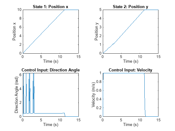
Simulate the system for two seconds with a target trajectory.

% Define the simulation duration in seconds.
Tf = 15;

% Initialize state and control vectors.
x0 = zeros(nx,1);
u0 = zeros(nmv,1);

% Preallocate history arrays to store states and control inputs
xHistory1 = x0.'; % State history
uHistory1 = u0.'; % Control input history

% Initialize the control input for the first step.
uk = u0;

% Use a for loop to simulate the system dynamics
% over the specified duration.
for k = 1:(Tf/Ts)
    % Set the current state at iteration k.
    xk = xHistory1(k,:).';
    
    % Compute the optimal control action using nlmpcmove.
    [uk,simdata,info] = nlmpcmove(msobj,xk,uk,simdata);
    
    % Simulate the system for the next control interval using ode45.
    odefun = @(t,xk) Navigation.StateFcn(xk,uk);
    [TOUT,XOUT] = ode45(odefun,[0 Ts],xk);
    
    % Log the states and control inputs for analysis and plotting.
    xHistory1(k+1,:) = XOUT(end,:);
    uHistory1(k+1,:) = uk;
end

Plot the state and control input histories.

% Set time vector for plotting.
time = 0:Ts:Tf;

figure;
tiledlayout(2,2);
ax = gobjects(4,1);
ax(1) = nexttile; plot(time,xHistory1(:,1))
ax(2) = nexttile; plot(time,xHistory1(:,2))
ax(3) = nexttile; plot(time,uHistory1(:,1))
ax(4) = nexttile; plot(time,uHistory1(:,2))

title(ax(1),"State 1: Position x")
title(ax(2),"State 2: Position y")
title(ax(3),"Control Input: Direction Angle")
title(ax(4),"Control Input: Velocity")

xlabel(ax,"Time (s)")
ylabel(ax(1),"Position x")
ylabel(ax(2),"Position y")
ylabel(ax(3),"Direction Angle (rad)")
ylabel(ax(4),"Velocity (m/s)")

Drift Navigation

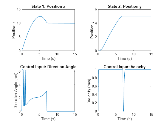
Adjust the state dynamics of the boat to account for drift.

msobj.Model.StateFcn = "Navigation.StateFcnWithDrift";
msobj.Model.StateJacFcn = "Navigation.StateJacFcnWithDrift";
simdata.InitialGuess = [];

Simulate the system for two seconds with a target trajectory.

% Preallocate arrays for storing states and control inputs.
xHistory2 = x0.'; % State history
uHistory2 = u0.'; % Control input history

% Initialize the control input for the first step.
uk = u0;

% Use a for loop to simulate the system dynamics
% over the specified duration.
for k = 1:(Tf/Ts)

    % Set the current state at iteration k.
    xk = xHistory2(k,:).';
    
    % Compute the optimal control action using nlmpcmove.
    [uk,simdata,info] = nlmpcmove(msobj,xk,uk,simdata);
    
    % Simulate the system for the next control interval using ode45.
    odefun = @(t,xk) Navigation.StateFcnWithDrift(xk,uk);
    [TOUT,XOUT] = ode45(odefun,[0 Ts],xk);
    
    % Log the states and control inputs for analysis and plotting.
    xHistory2(k+1,:) = XOUT(end,:);
    uHistory2(k+1,:) = uk;
end

Plot the state and control input histories.

figure;
tiledlayout(2,2);
ax = gobjects(4,1);
ax(1) = nexttile; plot(time,xHistory2(:,1));
ax(2) = nexttile; plot(time,xHistory2(:,2));
ax(3) = nexttile; plot(time,uHistory2(:,1));
ax(4) = nexttile; plot(time,uHistory2(:,2));

title(ax(1),"State 1: Position x");
title(ax(2),"State 2: Position y");
title(ax(3),"Control Input: Direction Angle");
title(ax(4),"Control Input: Velocity");

xlabel(ax,"Time (s)");
ylabel(ax(1),"Position x");
ylabel(ax(2),"Position y");
ylabel(ax(3),"Direction Angle (rad)");
ylabel(ax(4),"Velocity (m/s)");

Obstacle Avoidance

To enhance the capabilities of the MPC controller and ensure safe navigation, you can specify obstacle avoidance.

For this example, the obstacle is modeled as a circle, and its presence is within the MPC framework using inequality constraints. These constraints are defined by the Navigation.IneqConFcn and Navigation.IneqConJacFcn functions, which calculate the distance between the current position of the boat and the center of the obstacle; the boat is required to maintain a distance greater than the radius of the obstacle to avoid collision.

Update the msobj object to incorporate obstacle avoidance into each stage of the MPC controller. By assigning Navigation.IneqConFcn and Navigation.IneqConJacFcn to all stages of the MPC controller, you specify that the obstacle avoidance behavior for every prediction horizon step. Here, ParameterLength is set to 6 to account for the additional parameters required by these functions, which include the radius and center of the obstacle. This update equips the MPC controller with the necessary tools to navigate safely and efficiently in environments with static obstacles.

[msobj.Stages.IneqConFcn] = deal("Navigation.IneqConFcn");
[msobj.Stages.IneqConJacFcn] = deal("Navigation.IneqConJacFcn");
[msobj.Stages.ParameterLength] = deal(6);

Add obstacle avoidance parameters to the simulation data structure. Then validate the model functions.

pvcost = [xref; p; obs];
pvstate = 1;
simdata = getSimulationData(msobj);
simdata.StateFcnParameter = pvstate;
simdata.StageParameter = repmat(pvcost,p+1,1);
validateFcns(msobj,rand(nx,1),rand(nmv,1),simdata)

Model.StateFcn is OK.
Model.StateJacFcn is OK.
"CostFcn" of the following stages [1 2 3 4 5 6 7 8 9 10 11 12 13 14 15 16 17 18 19 20 21] are OK.
"CostJacFcn" of the following stages [1 2 3 4 5 6 7 8 9 10 11 12 13 14 15 16 17 18 19 20 21] are OK.
"IneqConFcn" of the following stages [1 2 3 4 5 6 7 8 9 10 11 12 13 14 15 16 17 18 19 20 21] are OK.
"IneqConJacFcn" of the following stages [1 2 3 4 5 6 7 8 9 10 11 12 13 14 15 16 17 18 19 20 21] are OK.
Analysis of user-provided model, cost, and constraint functions complete.

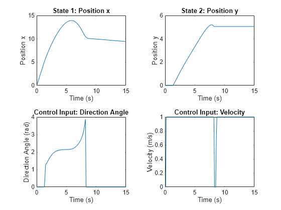
Perform a closed-loop simulation with obstacle avoidance.

% Preallocate arrays for storing states and control inputs.
xHistory3 = x0.'; % State history
uHistory3 = u0.'; % Control input history

% Initialize the control input for the first step.
uk = u0;

% Use a for loop to simulate the system dynamics
% over the specified duration.
for k = 1:(Tf/Ts)
    % Current state at iteration k.
    xk = xHistory3(k,:).';
    
    % Compute the optimal control action using nlmpcmove.
    [uk,simdata,info] = nlmpcmove(msobj,xk,uk,simdata);
    
    % Simulate the system for the next control interval using ode45.
    odefun = @(t,xk) Navigation.StateFcnWithDrift(xk,uk);
    [TOUT,XOUT] = ode45(odefun,[0 Ts],xk);
    
    % Log the states and control inputs for analysis and plotting.
    xHistory3(k+1,:) = XOUT(end,:);
    uHistory3(k+1,:) = uk;
end

Plot the state and control input histories.

figure;
tiledlayout(2,2);
ax = gobjects(4,1);
ax(1) = nexttile; plot(time,xHistory3(:,1));
ax(2) = nexttile; plot(time,xHistory3(:,2));
ax(3) = nexttile; plot(time,uHistory3(:,1));
ax(4) = nexttile; plot(time,uHistory3(:,2));

title(ax(1),"State 1: Position x");
title(ax(2),"State 2: Position y");
title(ax(3),"Control Input: Direction Angle");
title(ax(4),"Control Input: Velocity");

xlabel(ax,"Time (s)");
ylabel(ax(1),"Position x");
ylabel(ax(2),"Position y");
ylabel(ax(3),"Direction Angle (rad)");
ylabel(ax(4),"Velocity (m/s)");

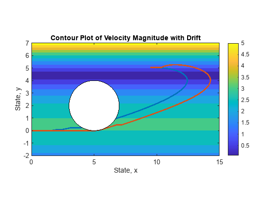
Plot the trajectories with (red) and without (blue) obstacle avoidance. Use the plotDriftVelocityMagnitude helper function (defined at the end of this example) to create a contour plot of velocity magnitude with drift. Here, the magnitude of the velocity is represented using a color scale from blue to yellow.

figure; 
plotDriftVelocityMagnitude(0,15,-2,7);

hold on; 
axis equal
plot(xHistory2(:,1),xHistory2(:,2),"LineWidth",2)
plot(xHistory3(:,1),xHistory3(:,2),"LineWidth",2)

theta = linspace(0,2*pi);
circle_x = obs(2) + obs(1)*cos(theta);
circle_y = obs(3) + obs(1)*sin(theta);
plot(circle_x,circle_y)
rectangle( ...
    "Position",[obs(2)-obs(1) obs(3)-obs(1) obs(1)*2 obs(1)*2], ...
    "Curvature",1, ...
    "FaceColor","w")

Figure contains an axes object. The axes object with title Contour Plot of Velocity Magnitude with Drift, xlabel State, x, ylabel State, y contains 5 objects of type contour, line, rectangle.

Helper Function to Create Contour Plot of Velocity with Drift

function plotDriftVelocityMagnitude(xlim1,xlim2,ylim1,ylim2)
% Create a contour plot of velocity magnitude with drift
%
%   plotDriftVelocityMagnitude(xlim1,xlim2,ylim1,ylim2) creates a
%   contour plot of the velocity magnitude with drift across a state
%   space defined by the limits xlim1, xlim2 for the x dimension and
%   ylim1, ylim2 for the y dimension. The function assumes 
%   no control inputs for demonstration.
%
%   Inputs:
%       xlim1 - Lower limit of the x dimension of the state space
%       xlim2 - Upper limit of the x dimension of the state space
%       ylim1 - Lower limit of the y dimension of the state space
%       ylim2 - Upper limit of the y dimension of the state space
%
%   Example:
%       plotDriftVelocityMagnitude(-5,5,-5,5)

% Copyright 2023 The MathWorks, Inc.

% Define a grid for the state space (x1 and x2).
x1_values = linspace(xlim1, xlim2); % Adjust these limits as needed.
x2_values = linspace(ylim1, ylim2); % Adjust these limits as needed.
[X1, X2] = meshgrid(x1_values, x2_values);

% Define control inputs (a and V)
a = 0; % Assuming zero angle for demonstration
V = 0; % Assuming zero velocity for demonstration

% Initialize the velocity field matrices.
Vx = zeros(size(X1)); % Velocity in the x-direction.
Vy = zeros(size(X2)); % Velocity in the y-direction.

% Loop over grid and compute velocity field from state function.
for i = 1:numel(X1)
    x = [X1(i); X2(i)]; % Current state
    u = [a; V];         % Control inputs
    pvstate = [];       % Placeholder

    % Evaluate the state function with drift.
    f = Navigation.StateFcnWithDrift(x, u, pvstate);

    % Store the resulting velocities.
    Vx(i) = f(1);
    Vy(i) = f(2);
end

% Compute the magnitude of the velocity vector at each point.
Vmag = sqrt(Vx.^2 + Vy.^2);

% Create the contour plot of the velocity magnitude.
contourf(X1, X2, Vmag, 'EdgeColor', 'none');
colorbar; % Add a color bar to indicate the magnitude scale
xlabel('State, x'); % Label for the x-axis
ylabel('State, y'); % Label for the y-axis
title('Contour Plot of Velocity Magnitude with Drift');
end

Solve Fuel-Optimal Navigation Problem Using C/GMRES

Problem Formulation

Design Nonlinear MPC Controller

Configure C/GMRES Solver

Closed-Loop Simulation in MATLAB

Drift Navigation

Obstacle Avoidance

Helper Function to Create Contour Plot of Velocity with Drift

See Also

Functions

Objects

Related Examples

More About