Control Underactuated Two-Link Robot Using C/GMRES Solver

This example uses:

This example shows how to control an underactuated two-link robot (commonly called a pendubot) using a Multistage Nonlinear Model Predictive Controller (NMPC) that solves the optimization problem with the C/GMRES solver.

Nonlinear Model

The Pendubot is an underactuated two-link planar robot with actuation only at the shoulder joint. The system is described by four state variables: two joint angles ( $θ_{1}$ and $θ_{2}$ ) and their respective angular velocities ( ${θ_{}^{˙}}_{1}$ and ${θ_{}^{˙}}_{2}$ ). The control input, $τ$ , is the torque applied at the shoulder joint.

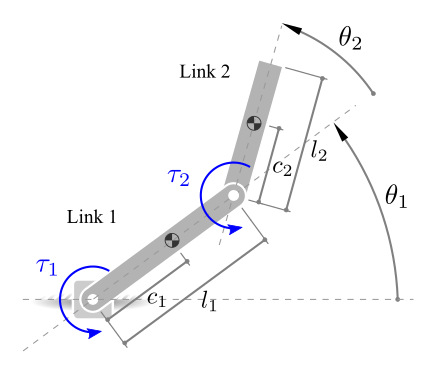
The state of the system consists of the joint angles and angular velocities $x = {[\begin{array}{cccc} θ_{1} & θ_{2} & {θ_{}^{˙}}_{1} & {θ_{}^{˙}}_{2} \end{array}]}^{T}$ .The system has one control input, $τ$ . The dynamics of the system are derived using Euler-Lagrange equations and include inertial, Coriolis, and gravitational terms.

This robot dynamics is implemented in Pendubot.stateFcn.m. This file is a MATLAB® function that takes as inputs the state vector, $x$ , the control input vector, $u$ , and a vector of model parameters, $pvstate = {[\begin{array}{cccccccc} d_{1} & d_{2} & l_{1} & m_{1} & m_{2} & J_{1} & J_{2} & g \end{array}]}^{T}$ . The function's output is the vector of the state derivatives with respect to time.

The physical parameters of the robot are defined in the following table:

Parameter	Value	Units	Description
$d_{1}$	0.15	$m$	Distance to the center of mass of the first link.
$d_{2}$	0.257	$m$	Distance to the center of mass of the second link.
$l_{1}$	0.3	$m$	Length of the first link.
$m_{1}$	0.2	$kg$	Mass of the first link.
$m_{2}$	0.7	$kg$	Mass of the second link.
$J_{1}$	0.006	${kgm}^{2}$	Moment of inertia of the first link.
$J_{2}$	0.051	${kgm}^{2}$	Moment of inertia of the second link.
$g$	9.80665	$m / s^{2}$	Gravitational acceleration.

Define model parameter vector:

pvstate = [0.15; 0.257; 0.3; 0.2; 0.7; 0.006; 0.051; 9.80665];

Control Objective

The control objective is twofold:

1. Swing-up Phase: Drive the robot from its stable downward equilibrium to the unstable upright equilibrium.

2. Stabilization Phase: Maintain both links upright ( $θ_{1} = π$ , $θ_{2} = 0$ ) with zero velocity.

Define initial state and reference state position:

% Initial state
x0 = zeros(4,1);    
% Reference state (upright position)
xref = [pi; 0; 0; 0];

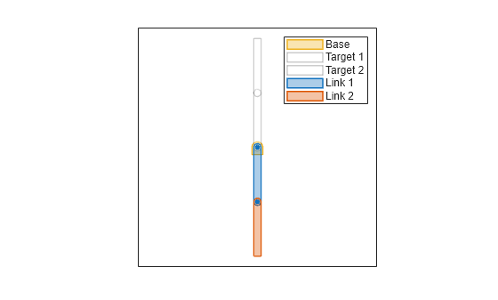
Create a custom chart object for animation, and use initial state and reference state position.

hPlot = RobotEnvironment( ...
    Length1 = pvstate(3), ...
    Length2 = pvstate(3));

% Set Initial angular position and desired state. 
hPlot.Theta1 = x0(1)-pi/2;
hPlot.Theta2 = x0(2);
hPlot.xf = xref - [pi/2;0;0;0];

Figure contains an object of type robotenvironment.

To achieve this, define a nonlinear cost function that penalizes deviations from the target state and large control inputs. For this example, the control strategy involves optimizing the performance index, $J$ , over a finite time horizon and is given by:

$J = \frac{1}{2} {‖ x (T) - x_{}^{‾} ‖}_{S_{f}}^{2} + \int_{t}^{t + T} \frac{1}{2} ({‖ x (t) - x_{}^{‾} ‖}_{Q}^{2} + {‖ u (t) ‖}_{R}^{2}) dt$

where:

$x_{}^{‾}$ represents the desired state.
$S_{f}$ , $Q$ , and $R$ are weight matrices that determine the importance of different terms in the performance index.

For this example, the weights and objective cost are implemented in the file Pendubot.m, where $S_{f} = Q = diag ([\begin{array}{cccc} 1 & 1 & 0.1 & 0.1 \end{array}])$ , and $R = 0.1$ .

Create Multistage NMPC Object

Create a nonlinear multistage MPC object with four states and one input.

% Create an NMPC object with 50 stages, 4 states, and 1 input
p = 50;
msobj = nlmpcMultistage(p,4,1);

% Set the control interval
msobj.Ts = 1/50;

% Specify the state transition function
msobj.Model.StateFcn = "Pendubot.stateFcn";
msobj.Model.StateJacFcn = "Pendubot.stateJacobianFcn";

% Set running cost for the Multistage NLMPC problem
[msobj.Stages(1:p).CostFcn] = deal("Pendubot.runningCostFcn");
[msobj.Stages(1:p).CostJacFcn] = deal("Pendubot.runningCostJacobianFcn");

% Set terminal cost for the Multistage NLMPC problem
msobj.Stages(p+1).CostFcn = "Pendubot.terminalCostFcn";
msobj.Stages(p+1).CostJacFcn = "Pendubot.terminalCostJacobianFcn";

% Specify number of parameters for model and stage functions
msobj.Model.ParameterLength = length(pvstate);
[msobj.Stages.ParameterLength] = deal(4);

Setting the Optimization Solver

For this example, set the multistage MPC object to use the cgmres solver.

msobj.Optimization.Solver = "cgmres";
msobj.Optimization.SolverOptions.MaxIterations = 5;
msobj.Optimization.SolverOptions.Restart = 0;
msobj.Optimization.SolverOptions.ConvergenceRate = 1.5;
msobj.Optimization.SolverOptions.ShootingMethod = "multiple-shooting";

Code Generation

Generate data structures using getCodeGenerationData.

[coredata, onlinedata] = getCodeGenerationData(msobj,x0,0, ...
    StateFcnParameter=pvstate, StageParameter=repmat(xref,p+1,1));

Generate a MEX function called nlmpcControllerMEX.

buildMEX(msobj, "nlmpcControllerMEX", coredata, onlinedata);

Generating MEX function "nlmpcControllerMEX" from your "nlmpcMultistage" object to speed up simulation.
Code generation successful.

MEX function "nlmpcControllerMEX" successfully generated.

Closed Loop Simulation

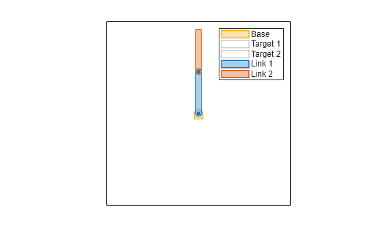
Simulate the closed-loop performance by integrating the plant forward in time using the state equations and applying the control input returned by the controller at each step.

FinalTime = 6;      % Simulation duration
x = x0;             % Initialize state
mv = 0;             % Initialize control input
Ts = 1e-3;          % Sampling time for simulation

% Initialize data storage
N = FinalTime/Ts;
tHistory = 0:Ts:FinalTime;
xHistory = zeros(N+1,4);
uHistory = zeros(N+1,1);

% Main simulation loop
for ct = 0:N
    % Compute optimal control move
    [mv,onlinedata,info] = nlmpcControllerMEX(x, mv, onlinedata);

    % Update plant state (Euler update)
    x = x + Pendubot.stateFcn(x,mv,pvstate)*Ts;

    % Store results
    xHistory(ct+1,:) = x;
    uHistory(ct+1,:) = mv;

    % Update underactuated two-link robot plot.
    hPlot.Theta1 = xHistory(ct+1,1)-pi/2;
    hPlot.Theta2 = xHistory(ct+1,2);
    drawnow limitrate
end

Figure contains an object of type robotenvironment.

Plot the joint angles over time to visualize the swing-up and stabilization behavior.

figure;
tiledlayout(2,2);
labels = {"\theta_1","\theta_2","\dot{\theta}_1","\dot{\theta}_2"};
for i=1:4
    nexttile(); 
    hold on;

    plot(0:Ts:FinalTime, xHistory(:,i)); 
    plot([0 FinalTime], [xref(i) xref(i)]);

    % Plot Settings
    xlabel("Time, s");
    title(sprintf("State %d",i));
    ylabel(sprintf("$%s(t)$",labels{i}),Interpreter="latex");
    legend(sprintf("$x_%d$",i),sprintf("$\\bar{x}_%d$",i),Interpreter="latex");
end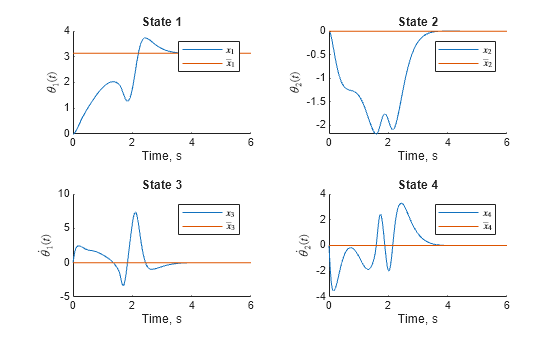

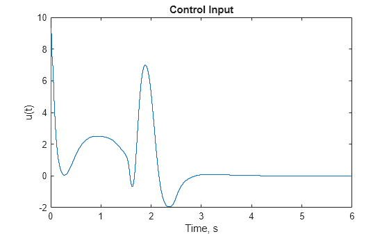
$Figure contains 4 axes objects. Axes object 1 with title State 1, xlabel Time, s, ylabel $\theta_1(t)$ contains 2 objects of type line. These objects represent $x_1$, $\bar{x}_1$. Axes object 2 with title State 2, xlabel Time, s, ylabel $\theta_2(t)$ contains 2 objects of type line. These objects represent $x_2$, $\bar{x}_2$. Axes object 3 with title State 3, xlabel Time, s, ylabel $\dot{\theta}_1(t)$ contains 2 objects of type line. These objects represent $x_3$, $\bar{x}_3$. Axes object 4 with title State 4, xlabel Time, s, ylabel $\dot{\theta}_2(t)$ contains 2 objects of type line. These objects represent $x_4$, $\bar{x}_4$.$

The pendubot swings up and stabilizes around the upright configuration within a few seconds. The MPC controller successfully handles the nonlinear, underactuated dynamics using only a single actuator.

figure;
stairs(0:Ts:FinalTime, uHistory);
title("Control Input");
xlabel("Time, s");
ylabel("u(t)");

Figure contains an axes object. The axes object with title Control Input, xlabel Time, s, ylabel u(t) contains an object of type stair.

References

[1] Ohtsuka, T. “Continuation/GMRES Method for Fast Algorithm of Nonlinear Receding Horizon Control.” Proceedings of the 39th IEEE Conference on Decision and Control (Cat. No.00CH37187), vol. 1, 2000, pp. 766–71 vol.1. IEEE Xplore, https://doi.org/10.1109/CDC.2000.912861.

Control Underactuated Two-Link Robot Using C/GMRES Solver

Nonlinear Model

Control Objective

Create Multistage NMPC Object

Setting the Optimization Solver

Code Generation

Closed Loop Simulation

References

See Also

Functions

Objects

Blocks

Topics