Generate Code to Plan and Execute Collision-Free Trajectories Using KINOVA Gen3 Manipulator
This example shows how to generate code in order to speed up planning and execution of closed-loop collision-free robot trajectories using model predictive control (MPC). For more information on how to use MPC for motion planning of robot manipulators, see the example Plan and Execute Collision-Free Trajectories Using KINOVA Gen3 Manipulator (Robotics System Toolbox).
Modifications for Code Generation
To enable code generation, adapt the code in Plan and Execute Collision-Free Trajectories Using KINOVA Gen3 Manipulator (Robotics System Toolbox) following the steps below.
Ensure all helper Nonlinear MPC functions are stored as separate program files instead of Anonymous Functions. This example requires the following helper files.
- Custom cost function: nlmpcCostFunctionKINOVACodeGen.m
- Custom inequality constraints: nlmpcIneqConFunctionKINOVACodeGen.m
- State function: nlmpcModelKINOVACodeGen.m
- Output function: nlmpcOutputKINOVACodeGen.m
- Jacobian of custom cost function: nlmpcJacobianCostKINOVACodeGen.m
- Jacobian of custom inequality constraints: nlmpcJacobianConstraintKINOVACodeGen.m
- Jacobian of state function: nlmpcJacobianModelKINOVACodeGen.m
- Jacobian of output function: nlmpcJacobianOutputKINOVACodeGen.m
Use the
Parametersproperty of thenlmpcmoveoptobject (and, when a mex file, theonlineDatastructure) to pass to the controller any parameter that might change at runtime (that is, at each time step) or between consecutive runs. For example, to enable the update of obstacles poses according to new sensor readings at each time step, the values of the current obstacle poses (posesNow) are added to theparamscell variable. Similarly, to update the target robot pose online, the target pose (poseFinal) is added to theParameterslist. All the parameters must be numerical values. At each time step, the updated value ofparamsis then copied into theParametersproperty of either thenlmpcmoveoptobject (ifnlmpcmoveis used) or in theonlineDatastructure (if a MEX file is used).Use
persistentvariables to pass in variables that are not numerical and are not externally modified at runtime. For example, therigidBodyTree(Robotics System Toolbox) objectrobotand the cell array ofcollisionMesh(Robotics System Toolbox) objectsworldare created and saved as persistent variables the first time a helper function is executed using the following code.
persistent robot world
if isempty(robot)
    robot = loadrobot('kinovaGen3', 'DataFormat', 'column');
    [world, ~] = helperCreateObstaclesKINOVA(posesNow);
end
Ensure all the functions used in helper files support code generation. For a list of built-in MATLAB® functions supported for code generation, see Functions and Objects Supported for C/C++ Code Generation (MATLAB Coder). To test if a custom function supports code generation, use
coder.screener(MATLAB Coder). For example, try runningcoder.screener('nlmpcIneqConFunctionKINOVA'). This example requires thatloadrobot(Robotics System Toolbox) andcheckCollision(Robotics System Toolbox) support code generation.Use
getCodeGenerationDataandbuildMEXto generate code for thenlmpcobject with the specified properties. Replacenlmpcmovein the original example with the generated MEX file to compute optimal control actions.
Robot Description and Poses
Load the KINOVA® Gen3 rigid body tree (RBT) model.
robot = loadrobot('kinovaGen3', 'DataFormat', 'column');
Get the number of joints.
numJoints = numel(homeConfiguration(robot));
Specify the robot frame where the end-effector is attached.
endEffector = "EndEffector_Link"; Specify initial and desired end-effector poses. Use inverse kinematics to solve for the initial robot configuration given a desired pose.
% Initial end-effector pose
taskInit = trvec2tform([0.4 0 0.2])*axang2tform([0 1 0 pi]);

% Compute current joint configuration using inverse kinematics
ik = inverseKinematics('RigidBodyTree', robot);
ik.SolverParameters.AllowRandomRestart = false;
weights = [1 1 1 1 1 1];
currentRobotJConfig = ik( ...
    endEffector, taskInit, weights, robot.homeConfiguration);
currentRobotJConfig = wrapToPi(currentRobotJConfig);

% Final (desired) end-effector pose
taskFinal = trvec2tform([0.35 0.55 0.35])*axang2tform([0 1 0 pi]);
anglesFinal = rotm2eul(taskFinal(1:3,1:3),'XYZ');

 % 6x1 vector for final pose: [x, y, z, phi, theta, psi]
poseFinal = [taskFinal(1:3,4);anglesFinal'];
Collision Meshes and Obstacles
To check for and avoid collisions during control, you must setup a collision world as a set of collision objects. This example uses collisionSphere (Robotics System Toolbox) objects as obstacles to avoid. To plan using static instead of moving objects, set isMovingObst to false.
isMovingObst = true;
The obstacle sizes and locations are initialized in the helperCreateMovingObstaclesKINOVACodeGen helper function. To add more static obstacles, add collision objects in the world array.
if isMovingObst == true
    helperCreateMovingObstaclesKINOVACodeGen
else
    posesNow = [0.4 0.4 0.25 ; 0.3 0.3 0.4];
end
[world, numObstacles] = ...
    helperCreateObstaclesKINOVACodeGen(posesNow);
Visualize the robot at the initial configuration. You should see the obstacles in the environment as well.
x0 = [currentRobotJConfig', zeros(1,numJoints)];
helperInitialVisualizerKINOVACodeGen;

Specify a safety distance away from the obstacles. This value is used in the inequality constraint function of the nonlinear MPC controller.
safetyDistance = 0.01;
Design Nonlinear Model Predictive Controller
You can design the nonlinear model predictive controller using the helperDesignNLMPCobjKINOVACodeGen helper file, which creates an nlmpc controller object. To view the file, at the MATLAB command line, enter edit helperDesignNLMPCobjKINOVACodeGen.
helperDesignNLMPCobjKINOVACodeGen;
Closed-Loop Trajectory Planning
Simulate the robot for a maximum of 50 steps with correct initial conditions.
Initialize Simulation Parameters
maxIters = 50;
u0 = zeros(1,numJoints);
mv = u0';
time = 0;
goalReached = false;
Generate Code for nlmpc Object
useMex = true;
buildMex = true;
if useMex
    [coredata, onlinedata] = getCodeGenerationData(nlobj,x0',u0',paras);
    if buildMex
        mexfcn = buildMEX(nlobj,'kinovaMex',coredata,onlinedata);
    end
end
Generating MEX function "kinovaMex" from nonlinear MPC to speed up simulation.
Code generation successful.

MEX function "kinovaMex" successfully generated.
Initialize Data Array for Control
positions = zeros(numJoints,maxIters);
positions(:,1) = x0(1:numJoints)';

velocities = zeros(numJoints,maxIters);
velocities(:,1) = x0(numJoints+1:end)';

accelerations = zeros(numJoints,maxIters);
accelerations(:,1) = u0';

timestamp = zeros(1,maxIters);
timestamp(:,1) = time;
Generate Trajectory
Use the generated MEX file kinovaMex instead of the nlmpcmove function to speed up closed-loop trajectory generation. Specify the trajectory generation online options using the argument onlineData.
Each iteration calculates the position, velocity, and acceleration of the joints to avoid obstacles as they move toward the goal. The helperCheckGoalReachedKINOVACodeGen script checks if the robot has reached the goal. The helperUpdateMovingObstaclesKINOVACodeGen script moves the obstacle locations based on the time step.
options = nlmpcmoveopt;

for timestep=1:maxIters
    disp(['Calculating control at timestep ', num2str(timestep)]);

    % Optimize next trajectory point
    if ~useMex
        options.Parameters = paras;
        [mv,options,info] = nlmpcmove(nlobj,x0,mv,[],[], options);
    else
        onlinedata.Parameters = paras;
        [mv,onlinedata,info] = kinovaMex(x0',mv,onlinedata);
    end

    if info.ExitFlag < 0
        disp('Failed to compute a feasible trajectory. Aborting...')
        break;
    end

    % Update states and time for next iteration
    x0 = info.Xopt(2,:);
    time = time + nlobj.Ts;

    % Store trajectory points
    positions(:,timestep+1) = x0(1:numJoints)';
    velocities(:,timestep+1) = x0(numJoints+1:end)';
    accelerations(:,timestep+1) = info.MVopt(2,:)';
    timestamp(timestep+1) = time;

    % Check if goal is achieved
    helperCheckGoalReachedKINOVACodeGen;
    if goalReached
        break;
    end

    % Update obstacle pose if it is moving
    if isMovingObst
        helperUpdateMovingObstaclesKINOVACodeGen;
    end
end
Calculating control at timestep 1
Calculating control at timestep 2
Calculating control at timestep 3
Calculating control at timestep 4
Calculating control at timestep 5
Calculating control at timestep 6
Calculating control at timestep 7
Calculating control at timestep 8
Target configuration reached.
Execute Planned Trajectory Using Low-Fidelity Robot Control and Simulation
Trim the trajectory vectors based on the time steps calculated from the plan.
tFinal = timestep+1;
positions = positions(:,1:tFinal);
velocities = velocities(:,1:tFinal);
accelerations = accelerations(:,1:tFinal);
timestamp = timestamp(:,1:tFinal);

visTimeStep = 0.2;
Use a jointSpaceMotionModel object to track the trajectory with computed-torque control. The helperTimeBasedStateInputsKINOVA function generates the derivative inputs for the ode15s ODE solver to simulate the robot movement along the computed trajectory.
% specify low-fidelity model
motionModel = jointSpaceMotionModel('RigidBodyTree', robot);

% Specify initial and target states
initState = [positions(:,1);velocities(:,1)];
targetStates = [positions;velocities;accelerations]';

% Control robot to track trajectory points in simulation
[t,robotStates] = ode15s(@(t,state) ...
    helperTimeBasedStateInputsKINOVA( ...
        motionModel, timestamp, targetStates, t, state), ...
        timestamp(1):visTimeStep:timestamp(end), initState);
Visualize the robot motion.
helperFinalVisualizerKINOVACodeGen;
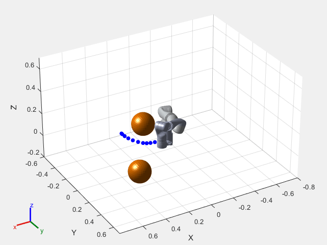
As expected, the robot successfully moves along the planned trajectory and avoids the obstacles.
See Also
Functions
Objects
Blocks
Topics
- Plan and Execute Collision-Free Trajectories Using KINOVA Gen3 Manipulator (Robotics System Toolbox)
- Nonlinear MPC