Offroad Planning with Digital Elevation Models

Open Live Script

This example shows how to process and store 2.5-D information, and presents various techniques for using it for an offroad path planner.

Mobile robot planning often involves finding the shortest path for a wheeled robot in the presence of obstacles. Planners often assume that the planning space is a 2-D Cartesian plane, with certain regions marked as off limits due to the presence of obstacles. When it comes to offroad vehicles, environments can also contain changes in elevation, turning this into a three-dimensional problem. Planning in higher-dimension spaces coincides with longer planning times, so an effective compromise can be to plan in a 2.5-D space using Digital Elevation Models (DEMs). This example shows the process of creating and testing planning heuristics in simulation, and then shows how to apply those heuristics to achieve 2.5-D path planning for an offroad planner with real-world data. In this example, you will use

A-Star path planner for wheeled mobile robots
Hybrid A-Star path planner for car-like robots

Define Planning Space

Create Planning Surface

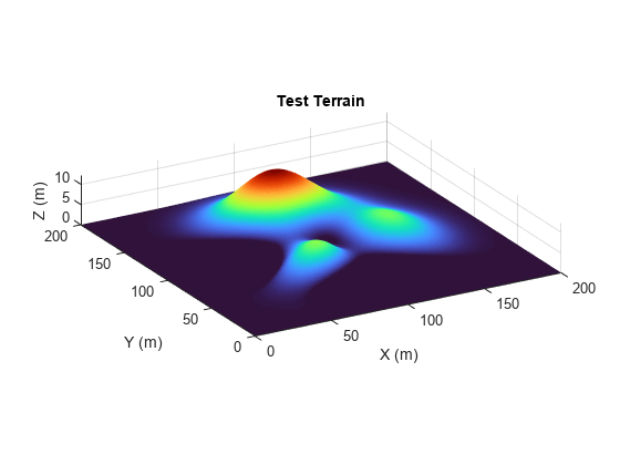
Most environment models are created from sensors mounted on the robot, or retrieved from a database based on the estimated pose of the platform. Create a surface using peaks to act as the environment model to test the effect of different cost functions for the planner.

% Add helper folders to path
addpath("Analysis","Data","Heuristics","MapProcessing");

% Create surface
[X,Y] = meshgrid(-100:100);
Z = peaks(max(size(X)))*1.5; % Units in meters
X = X + 100;                 % Move X origin from center to corner
Y = Y + 100;                 % Move X origin from center to corner
Z(Z<0) = 0;                  % Discard valleys

% Visualize surface
figure
ax = gca;
surf(ax,X,Y,Z,EdgeColor="none")
title("Test Terrain")
xlabel("X (m)")
ylabel("Y (m)")
zlabel("Z (m)")
colormap("turbo")
ax.PlotBoxAspectRatio = [1 1 0.15];
view([-29.59 21.30])

Define Heuristics for 2.5-D Space

Next, define the heuristics. These heuristics utilize elevation data in different ways to create a cost, $C$ , which may result in improvement versus path planning in only two dimensions:

exampleHelperZHeuristic

This cost function augments the planning state (XY) with the surface height (Z) before calculating distance. This should result in the shortest possible route through the 2.5-D manifold, balancing changes in elevation against distance to find the most direct path between two points:

$C_{Z} = | | {s^{*}}_{2} - {s^{'}}_{1} | |$ , where ${s^{*}}_{i} = [x_{i} y_{i} z_{i} * w]$ ,

exampleHelperGradientHeuristic

This cost function adds a cost that scales with the steepness of the slope in the same direction as the heading. Unlike the Z heuristic, this penalty is not scaled by distance, and should therefore bias the planner towards routes that minimize immediate changes in elevation, potentially saving energy:

$C_{Slope} = {\begin{cases} | | s_{2} - s_{1} | | + w * ⟨ \hat{| s_{2} - s_{1} |}, | g_{x} g_{y} | ⟩ & if slope < {slope}_{\max} \\ e^{⟨ \hat{| s_{2} - s_{1} |}, | g_{x} g_{y} | ⟩} & else \end{cases}$

exampleHelperRolloverHeuristic

This cost function is similar to exampleHelperGradientHeuristic, but by flipping the X and Y values of the spatial gradient, it penalizes motions whose direction is perpendicular to the slope. In other words, this function should minimize the risk of rollover by seeking routes with low roll angles:

$C_{Roll} = {\begin{cases} | | s_{2} - s_{1} | | + w * ⟨ \hat{| s_{2} - s_{1} |}, | g_{y} g_{x} | ⟩ & if slope < {slope}_{\max} \\ e^{⟨ \hat{| s_{2} - s_{1} |}, | g_{y} g_{x} | ⟩} & else \end{cases}$

Each cost function includes a weighting variable that scales the accompanying heuristic. You can adjust the weight to prioritize the quickest 2-D route (weight = 0) or a potentially more energy-efficient path (weight = 4).

Discretize and Store Environment Information in Map Layers

With the cost functions defined, we know what information to retrieve from the environment. Discretely sample the 3-D surface and store the results in mapLayer objects. These provide transforms between Cartesian coordinates and functions for querying or modifying data, similar to the binaryOccupancyMap and occupancyMap objects.

Construct Z-Layer

You can take the height layer directly from the surface and store it in a mapLayer object, effectively serving as your Digital Elevation Model. Create a map layer to contain the height of the surface with ground clutter and obstacles removed.

% Query and store the Z-height
zLayer = mapLayer(flipud(Z),LayerName="Z");

Calculate Gradients and Convert to Cost

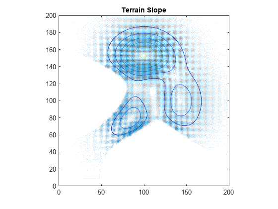
Calculate the gradient and cost information from the Z-layer. First, calculate the X and Y gradients of the surface, and use the contour function to visualize the gradients as a contour map.

[gx,gy] = gradient(Z);
figure
contour(X,Y,Z)
title("Terrain Slope")
hold on
quiver(X,Y,gx,gy)
axis equal
hold off

Store the X and Y gradients in mapLayer objects.

dzdx = mapLayer(flipud(gx),LayerName="dzdx");
dzdy = mapLayer(flipud(gy),LayerName="dzdy");

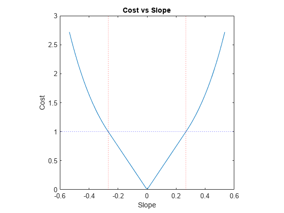
Define the function exampleHelperGradientToCost, which maps gradient values to a cost. To make it more intuitive to apply a cost-weighting variable, use slopes to determine the cost weighting. Slope values from 0 to a maximum slope scale linearly in the range [0 1], and values larger than the maximum slope scale exponentially:

$C = {\begin{cases} \frac{| m |}{m_{\max}} & , 0 \leq | m | \leq m_{\max} \\ e^{(\frac{| m |}{m_{\max}} - 1)} & , m_{\max} \leq | m | \end{cases},$

where $m$ is slope. Define the maximum incline angle as 15 degrees, and convert this to the maximum slope.

maxinclineangle = 15; % Degrees
maxSlope = tand(maxinclineangle); % Max preferred slope for vehicle

Visualize the unweighted slope-to-cost function.

slope2cost = @(x)exampleHelperGradientToCost(maxSlope,flipud(x));
slope = linspace(-2*maxSlope,2*maxSlope,100);
plot(slope,slope2cost(slope))
hold on
xline(maxSlope*[-1 1],"r:")
yline(1,"b:")
title("Cost vs Slope")
xlabel("Slope")
ylabel("Cost")
axis square

Calculate costs using the slope function, and store them in map layers.

xCost = mapLayer(slope2cost(gx),LayerName="xCost");
yCost = mapLayer(slope2cost(gy),LayerName="yCost");
diagCost = mapLayer(slope2cost(sqrt(gx.^2+gy.^2)),LayerName="diagCost");

Terrain Obstacles

In addition to elevation and slope information, you must represent areas that are off limits, either due to high slope or obstacles. Use binaryOccupancyMap or occupancyMap objects to represent such regions for a plannerAStarGrid planner.

Generate a random matrix, then mark all elements with values above a specified threshold as obstacle locations. To represent the obstacle probabilities for testing, set the obstacle probabilities to random values.

rng(4) % Set RNG seed for repeatable results
obstacleprob = rand(max(size(X)));

Create a binaryOccupancyMap containing the obstacles and inflated terrain.

obstacleMap = binaryOccupancyMap(flipud(obstacleprob>0.998),LayerName="obstacles");
terrainObstacles = binaryOccupancyMap(obstacleMap,LayerName="terrainObstacles");
inflate(terrainObstacles,2);

Check each cell against the three slope constraints, and block off cells that violate all three slope constraints.

obstaclesAndTerrain = double(getMapData(terrainObstacles));
mInvalidSlope = getMapData(xCost) > 1 & getMapData(yCost) > 1 & getMapData(diagCost) > 1;
obstaclesAndTerrain(mInvalidSlope) = true;
setMapData(terrainObstacles,obstaclesAndTerrain);

Display a map containing the raw obstacles and a map containing inflated obstacles and invalid terrain.

figure
show(obstacleMap,Parent=subplot(1,2,1))
show(terrainObstacles,Parent=subplot(1,2,2))
title("Obstacles and Gradient-Restricted Regions")

Combine Individual Map Layers

To organize your data and keep your layers synchronized, add your layers to a multiLayerMap. This ensures that updating shared properties of one layer also updates the others, so that the data always represents the same region of Cartesian space.

costMap = multiLayerMap({zLayer dzdx dzdy terrainObstacles obstacleMap xCost yCost diagCost});

Make maps egocentric by updating the GridOriginInLocal value of the X cost map, and then restore the map to its original settings.

xCost.GridOriginInLocal = -xCost.GridSize/xCost.Resolution/2

xCost = 
  mapLayer with properties:

   mapLayer Properties
               DataSize: [201 201]
               DataType: 'double'
           DefaultValue: 0
               GridSize: [201 201]
              LayerName: 'xCost'
    GridLocationInWorld: [-100.5000 -100.5000]
      GridOriginInLocal: [-100.5000 -100.5000]
     LocalOriginInWorld: [0 0]
             Resolution: 1
           XLocalLimits: [-100.5000 100.5000]
           YLocalLimits: [-100.5000 100.5000]
           XWorldLimits: [-100.5000 100.5000]
           YWorldLimits: [-100.5000 100.5000]
        GetTransformFcn: []
        SetTransformFcn: []

% Restore map to original settings
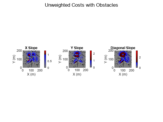
costMap.GridOriginInLocal = [0 0];

Visualize obstacles on top of the three slope-based cost layers. In these graphs, note how the slope threshold affects the cost:

Gray — Free space
Shades of blue — Varying costs below the soft threshold (the closer to gray, the lower the cost)
Shades of red — Varying costs above the soft threshold (brighter red, higher cost)
Black — Obstacles and cells that violate the slope threshold in all directions

figure(5)
obstaclesAndTerrain(obstaclesAndTerrain < 1) = nan; % Turn 0s to NaNs for plotting on costmaps

show(visualizationHelper,xCost,subplot(1,3,1),hold="on",title="X Slope",Threshold=1);
surface(flipud(obstaclesAndTerrain),FaceColor=[0 0 0])

show(visualizationHelper,yCost,subplot(1,3,2),hold="on",title="Y Slope",Threshold=1);
surface(flipud(obstaclesAndTerrain),FaceColor=[0 0 0])

show(visualizationHelper,diagCost,subplot(1,3,3),hold="on",title="Diagonal Slope",Threshold=1);
surface(flipud(obstaclesAndTerrain),FaceColor=[0 0 0])
sgtitle("Unweighted Costs with Obstacles")

Plan Paths Using 2.5-D Heuristics

Create Planners

Create a set of planners, each using one of the defined heuristics, and compare their planning results. Select the planner type as

plannerAStarGrid for wheeled mobile robots.
plannerHybridAStar for car-like robots.

plannerType = "plannerAStarGrid"

plannerType = 
"plannerAStarGrid"

Specify the start and goal poses in world coordinates.

start = [54 131 pi/3];
goal  = [143 104 pi/3];

If the planner type is plannerAStarGrid, convert the start and goal locations to grid coordinates.

if strcmp(plannerType,"plannerAStarGrid")
    start = world2grid(costMap,start(:,1:2));
    goal  = world2grid(costMap,goal(:,1:2));
end

Use the exampleHelperCreatePlannerObject helper function to create variations of the specified path planner. If you specify plannerAStarGrid as the path planner, the exampleHelperCreatePlannerObject function computes Z heuristics, gradient heuristics and rollover heuristics using the gWeight and hweight parameters.

If you specify plannerHybridAStar as the path planner, the exampleHelperCreatePlannerObject function computes Z heuristics, gradient heuristics and rollover heuristics using the gWeight parameter.

gWeight and hWeight are custom cost function parameters that determine the priority of nodes during the search process.

gWeight represents the weight or cost of the path from the start node to the current node. Increase this value to minimize the actual distance traveled and to prioritize finding shorter path between the start pose and goal pose.
hWeight represents the estimated cost or heuristic value from the current node to the goal node. Increase this value to minimize the estimated distance to the goal pose and to prioritize finding paths that are closer to the goal.

The combination of these weights guide the planner towards finding an optimal path based on the priority.

gWeight = 1;
hWeight = 1;
[defaultPlanner,heightAwarePlanner,gradientAwarePlanner,rolloverAwarePlanner] = exampleHelperCreatePlannerObject(plannerType,costMap,gWeight,hWeight);

Plan Paths

Plan the paths with each heuristic from the start to the goal and store them in a cell array. Use tic and toc to measure the time it takes for each heuristic planner to plan their path.

% Planners return a sequence of IJ cells
paths = cell(4,1);
pathNames = ["Default","Elevation-Aware Path","Gradient-Aware Path","Rollover-Aware Path"];
planningTime = nan(4,1);
tic;
paths{1} = plan(defaultPlanner,start,goal);
planningTime(1) = toc;
paths{2} = plan(heightAwarePlanner,start,goal);
planningTime(2) = toc-planningTime(1);
paths{3} = plan(gradientAwarePlanner,start,goal);
planningTime(3) = toc-planningTime(2);
paths{4} = plan(rolloverAwarePlanner,start,goal);
planningTime(4) = toc-planningTime(3);

if strcmp(plannerType,"plannerHybridAStar")
    for i=1:4 %#ok<UNRCH>
        paths{i} = paths{i}.States;
    end
end

Compare and Analyze Results

Compare the performance of each planner by defining a set of metrics and visualizing the motion along each path. This example models the platform as a simple ground vehicle, and makes some simplifying assumptions related to the energy required to operate the robot. Edit these parameters to see how the planning results are affected.

Define Robot and Scenario Parameters

% Define simulation parameters
scenarioParams.Gravity = 9.81;    % m/s^2
scenarioParams.UpdateRate = 1/60; % Hz

% Define vehicle parameters for estimating power consumption
scenarioParams.Robot.Mass = 70;     % kg, no payload
scenarioParams.Robot.Velocity = 0.6; % m/s
scenarioParams.Robot.AmpHour = 24;   % A-hr
scenarioParams.Robot.Vnom = 24;                             % V, Voltage
scenarioParams.Robot.RegenerativeBrakeEfficiency = 0;

Define Performance Metrics

For the analysis, use 3-D path distance, travel time, planning time, and energy expenditure as a rough measure of path efficiency. Also define the minimum, maximum, and average pitch and roll angles of the vehicle, to compare the relative quality of each path. For more information, see exampleHelperCalculateMetrics.

% Display result
figure
animateResults = true;
statTable = exampleHelperCalculateMetrics(costMap,scenarioParams,paths,planningTime,pathNames,plannerType)

statTable=4×8 table
                            Distance (m)    Power (W)    Travel Time (s)    Planning Time (s)    Max Pitch (deg)    Average Pitch (deg)    Max Roll (deg)    Average Roll (deg)
                            ____________    _________    _______________    _________________    _______________    ___________________    ______________    __________________

    Default                     101.2        226.85          2.8112             0.031432             13.744               6.4108               18.797              7.4844      
    Elevation-Aware Path        100.7        218.13          2.7972               2.5137             12.274               4.1055               14.542              3.9993      
    Gradient-Aware Path        100.71        218.13          2.7975                7.038             11.702               4.1577                 7.79              2.2989      
    Rollover-Aware Path        100.85        218.64          2.8013               5.5414             14.751               4.7195               4.4032             0.78052

Visualize the path results using exampleHelperVisualizeResults. This helper function projects all of the previously generated paths onto the 3-D surface.

exampleHelperVisualizeResults(gca,statTable,scenarioParams,costMap,paths,pathNames,~animateResults,plannerType);

Visualize Path Results

Visualize the robot following each of the planned paths.

figure
exampleHelperVisualizeResults(gca,statTable,scenarioParams,costMap,paths,pathNames,animateResults,plannerType);

Analyzing the results, the elevation-aware planner offers the best result for the lowest 3-D distance and time, and keeps power consumption relatively low, but the elevation-aware planner does little to steer the robot away from regions with steep inclines or high roll angles. The default planner also takes a short route, even with height included in the distance metric, but it expends additional energy ascending and descending slopes that the elevation-aware planner avoids, resulting in a higher power consumption.

The gradient-based planners trade distance and time for safer routes that consume less power compared to the other planners. The gradient-aware planner minimizes the time spent climbing and descending hills, whereas the rollover-aware planner seeks a path that keeps it level while traversing terrain. These results are reflected in the pitch and roll metrics, where the gradient-aware planner shows the lowest average pitch, and the rollover-aware planner shows maximum and average roll angles well below the other planners.

Plan on Real-World Digital Elevation Model Data

Now that you have tested the heuristics on an artificial surface, test them using real-world elevation data.

Import Real-World Data

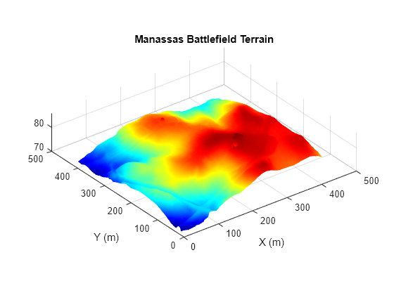
You can import Digital Elevation Data from a variety of sources. This example uses a TIF file downloaded from USGS National Land Cover Database that contains elevation data for Manassas National Battlefield Park, Virginia in the US. If you want to download this file yourself, follow these steps:

In the database address bar, search "Manassas National Battlefield Park, VA".
Zoom to the region of interest.
On the Datasets tab, under Data, select Elevation Products (3-DEP) > 1 meter DEM, and click Search Products.
Download the file covering the region for which you want elevation data.

Once downloaded, you can extract the elevation data from the TIF file using the readgeoraster function of Mapping Toolbox™:

Note: This code requires Mapping Toolbox

% Load the terrain data 
[elevation,info] = readgeoraster("USGS_1m_x28y430_VA_Fairfax_County_2018.tif",OutputType="double");
res = 2.5;

% Select a portion of the terrain data
Zinit = flipud(elevation(700:1100,800:1200));
[Xinit,Yinit] = meshgrid(1:length(Zinit));

% Interpolate for better matching with image resolution
[Xreal,Yreal] = meshgrid(1:(1/res):length(Zinit));
Zreal = interp2(Xinit,Yinit,Zinit,Xreal,Yreal);

For this example, the data has been processed for you and stored in a MAT file. Load the post-processed data for the subregion of interest.

% Load saved surface data and resolution
load("manassasData.mat");

% Visualize surface
surf(Xreal,Yreal,Zreal,EdgeColor="none")
formatAxes(visualizationHelper,title="Manassas Battlefield Terrain",colormap="jet")
pbaspect([1 1 0.2])

Load satellite imagery of the same location

img = imread("visitorcenter_satellitesq.jpg");
imgResized = imresize(img,[1001 1001]);
imshow(img)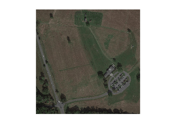

Create Data Layers

Repeat the same process as in the Calculate Gradients and Convert to Cost section to create the gradient and gradient cost layers.

figure
[gxReal,gyReal] = gradient(Zreal);
contour(Xreal,Yreal,Zreal)
formatAxes(visualizationHelper,title="Terrain Slope",hold="on",colormap="jet")
quiver(Xreal,Yreal,gxReal,gyReal)

Convert the satellite image into a terrain-obstacle map.

% Construct data layers
zLayerReal = mapLayer(flipud(Zreal),Resolution=res,LayerName="Z");
dzdxReal = mapLayer(flipud(gxReal),Resolution=res,LayerName="dzdx");
dzdyReal = mapLayer(flipud(gyReal),Resolution=res,LayerName="dzdy");
xCostReal = mapLayer(slope2cost(flipud(gxReal)),Resolution=res,LayerName="xCost");
yCostReal = mapLayer(slope2cost(flipud(gyReal)),Resolution=res,LayerName="yCost");
diagCostReal = mapLayer(slope2cost(flipud(sqrt(gxReal.^2+gyReal.^2))),Resolution=res,LayerName="diagCost");

Because an overhead satellite image is available, you can attempt to apply cost or invalidate areas of the map based on the absence or presence of vegetation. Use three filters: one to highlight colors with low spectral intensity (roads), another that focuses on greens (open fields), and a third that highlights browns and yellows (tall grass).

% Use thresholding to segment the image
[BWroads,roadRGB] = exampleHelperHighlightRoad(imgResized);
[BWfields,fieldRGB] = exampleHelperHighlightField(imgResized);
[BWbrush,brushRGB] = exampleHelperHighlightBrush(imgResized);
figure
imshow(roadRGB,Parent=subplot(1,3,1))
title("Tarmac")
imshow(fieldRGB,Parent=subplot(1,3,2))
title("Low Grass")
imshow(brushRGB,Parent=subplot(1,3,3))
title("High Brush")

Combine these three maps to create a terrain effort cost with the following weights for each type of terrain:

Road or Tarmac — 0
Low Grass — 1
High Brush — 3

Count the number of these categories for which each cell qualifies, and calculate the cost for each cell.

count = double(BWroads) + double(BWfields) + double(BWbrush);
terrainCost = (double(BWfields) + double(BWbrush)*3)./count;

Replace NaN values with values interpolated from neighbors.

[ii,jj] = meshgrid(1:size(terrainCost,1),1:size(terrainCost,2));
inan = isnan(terrainCost);
terrainCost(inan) = max(griddata(ii(~inan),jj(~inan),terrainCost(~inan),ii(inan),jj(inan),"linear"),0);

For simplicity, this example marks any terrain with a slope or surface cost over a given threshold as occupied, but these costs could be incorporated into existing or new cost functions as well.

Insert the terrain costs into a layer and define a maximum terrain cost. Changing the maximum terrain cost can affect what terrain the binary occupancy map sees as an obstacle.

terrainLayer = mapLayer(terrainCost,Resolution=res,LayerName="surfaceCost");
maxTerrainCost = 2.5;

Convert the terrain costs into a binaryOccupancyMap object.

terrainObstaclesReal = binaryOccupancyMap(terrainLayer.getMapData >= maxTerrainCost,Resolution=res,LayerName="terrainObstacles");

Inflate slope-blocked cells and set them as obstacles.

inflate(terrainObstaclesReal,.25);
terrainData = getMapData(terrainObstaclesReal);
mInvalidSlope = getMapData(xCostReal) > 1 & getMapData(yCostReal) > 1 & getMapData(diagCostReal) > 1;
terrainData(mInvalidSlope) = true;
setMapData(terrainObstaclesReal,terrainData);

Display the terrain costs and occupancy map side-by-side.

figure
show(visualizationHelper,terrainLayer,subplot(1,2,1),title="Terrain Surface Cost",Threshold=maxTerrainCost)
show(terrainObstaclesReal,Parent=subplot(1,2,2))

Combine the cost map layers into a multiLayerMap object.

costMapReal = multiLayerMap({zLayerReal dzdxReal dzdyReal terrainObstaclesReal xCostReal yCostReal diagCostReal});

Define start and goal positions in world coordinates.

start = [290 300];
goal = [95 165];

Create a planning configuration by configuring the custom cost functions. Explore how different configurations impact the planned path.

Plan Path Using `plannerHybridAstar`

Hybrid A-Star with default transition cost tCostType and default analytical expansion cost aeCostType is useful for planning an optimal and feasible path for a Car-like robot in the presence of obstacles in a structured environment. Height and road surface quality must also be considered when planning an optimal path in an uneven road or off-road. This can be accomplished by selecting custom tCostType or aeCostType.

Configure Transition Cost Function

The function set to the TransitionCostFcn property of plannerHybridAStar calculates the distance traveled (or cost) between two poses in the planning graph.

    tCostType = "tDefault";
    transFcnChoices = exampleHelperHybridAStarFcnOptions("Function Type",tCostType);
    tWeightRange    = exampleHelperHybridAStarFcnOptions("Weight Range",tCostType);
    tWLow  = tWeightRange(1);
    tWHigh = tWeightRange(2);
    tStep  = tWeightRange(3);
    tWeight = 1;
    vArgs = exampleHelperHybridAStarFcnOptions("Cost Function Inputs",tCostType);
    tCostSetting = exampleHelperHybridAStarFcnOptions("Function Selection",transFcnChoices(1),vArgs{:});

Configure Analytical Expansion Cost Function

The function set to the AnalyticalExpansionCostFcn property of plannerHybridAStar calculates the Reeds-Shepp connection from current pose to goal pose. This is the last segment of the actual path of plannerHybridAStar.

    aeCostType = "aeDefault";
    aeFcnChoices = exampleHelperHybridAStarFcnOptions("Function Type", aeCostType);
    aeWeightRange = exampleHelperHybridAStarFcnOptions("Weight Range",  aeCostType);
    aeWLow = aeWeightRange(1);
    aeWHigh = aeWeightRange(2);
    aeStep = aeWeightRange(3);
    aeWeight = 1;

    vArgs = exampleHelperHybridAStarFcnOptions("Cost Function Inputs",aeCostType);
    aeCostSetting = exampleHelperHybridAStarFcnOptions("Function Selection",aeFcnChoices(1), vArgs{:});

Create plannerHybridAStar object for the selected cost functions.

% Create a stateValidator object
map = getLayer(costMapReal,"terrainObstacles");
validator = validatorOccupancyMap;

% Assigning map to stateValidator object
validator.Map = map;

validator.StateSpace.StateBounds = [map.XLocalLimits; map.YWorldLimits; [-pi pi]];

pHybridAStarObj = plannerHybridAStar(validator,tCostSetting{:},aeCostSetting{:});

Add heading angles to the start and goal positions in order to plan path using Hybid-A* planner.

startPose = [start pi/3];
goalPose  = [goal pi/3];

tic;
hybridAStarPathRealObj = plan(pHybridAStarObj,startPose,goalPose);
hybridAStarPlanningTimeReal = toc;

hybridAStarPathReal = hybridAStarPathRealObj.States;

Plan Path Using `plannerAStarGrid`

Configure G-Cost Function

The function set to the GCostFcn property of plannerAStarGrid calculates the distance traveled (or cost) between two nodes in the planning graph. The planner then adds this cost to the accumulated cost between the root node and the current node to form the g-cost:

$g_{{cost}_{i}} = \sum_{n = 0}^{i - 1} g_{{node}_{n - 1}, {node}_{n}} + gCostFcn ({node}_{i - 1}, {node}_{i})$

gCostType = "gDefault";
gFcnChoices = exampleHelperFcnOptions("Function Type",gCostType);
gWeightRange = exampleHelperFcnOptions("Weight Range",gCostType,"g");
gWLow = gWeightRange(1);
gWHigh = gWeightRange(2); 
gStep = gWeightRange(3);
gWeight = 1;
vArgs = exampleHelperFcnOptions("Cost Function Inputs",gCostType);
gCostSetting = exampleHelperFcnOptions("Function Selection",gFcnChoices(1),vArgs{:});

Configure H-Cost Function

The hCostFcn of the planner calculates the cost-to-go, or estimated cost, between the current node and the goal node. The h-cost serves as a heuristic to guide the planner during exploration. In order to satisfy the optimality guarantee of A*, it should also be an underestimate of the cost-to-go:

$h_{{cost}_{i}} = hCostFcn ({node}_{i}, {node}_{goal})$

hCostType = "hDefault";
hFcnChoices = exampleHelperFcnOptions("Function Type",hCostType);
hWeightRange = exampleHelperFcnOptions("Weight Range",hCostType);
hWLow = hWeightRange(1);
hWHigh = hWeightRange(2);
hStep = hWeightRange(3);
hWeight = 1;
vArgs = exampleHelperFcnOptions("Cost Function Inputs",hCostType);
hCostSetting = exampleHelperFcnOptions("Function Selection",hFcnChoices(1),vArgs{:});

Add the g-cost and h-cost together to calculate the f-cost. The A* planner uses the f-cost to prioritize the next node to explore in the graph:

$f_{{cost}_{i}} = g_{{cost}_{i}} + h_{{cost}_{i}}$

Construct the A* planner with the selected cost functions.

pAStarGridObj = plannerAStarGrid(getLayer(costMapReal,"terrainObstacles"),hCostSetting{:},gCostSetting{:});

Convert start and goal positions to grid coordinates. Then, plan a path between the start and goal positions.

startPosition = world2grid(costMapReal,start);
goalPosition = world2grid(costMapReal,goal);

tic;
aStarGridPathReal = plan(pAStarGridObj,startPosition,goalPosition);
aStarGridPlanningTimeReal = toc;

Compare and Analyze Results

Compare the performance of planners plannerHybridAStar and plannerAStarGrid by computing these metrics: 3-D path distance, travel time, planning time, and energy expenditure. These metrics are approximate indicators of path efficiency. Additionally, use the maximum pitch, average pitch and roll angles of the vehicle to assess and compare the relative quality of each path. Visualize the motion along each path.

Edit the robot and scenario parameters to see how the planning results and the metrics are affected.

Define Robot and Scenario Parameters

% Define simulation parameters
scenarioParams.Gravity = 9.81;    % m/s^2
scenarioParams.UpdateRate = 1/60; % Hz

% Define vehicle parameters for estimating power consumption
scenarioParams.Robot.Mass = 70;     % kg, no payload
scenarioParams.Robot.Velocity = 0.6; % m/s
scenarioParams.Robot.AmpHour = 24;   % A-hr
scenarioParams.Robot.Vnom = 24;                             % V, Voltage
scenarioParams.Robot.RegenerativeBrakeEfficiency = 0;

Define Performance Metrics

hybridAStarStatTableReal = exampleHelperCalculateMetrics(costMapReal,scenarioParams,hybridAStarPathReal,hybridAStarPlanningTimeReal,"Hybrid A-Star Planner","plannerHybridAStar")

hybridAStarStatTableReal=1×8 table
                             Distance (m)    Power (W)    Travel Time (s)    Planning Time (s)    Max Pitch (deg)    Average Pitch (deg)    Max Roll (deg)    Average Roll (deg)
                             ____________    _________    _______________    _________________    _______________    ___________________    ______________    __________________

    Hybrid A-Star Planner       262.83        197.68          7.3009               7.419              2.4935               0.65724              1.8676             0.74708

astarGridStatTableReal = exampleHelperCalculateMetrics(costMapReal,scenarioParams,aStarGridPathReal,aStarGridPlanningTimeReal,"A-Star Grid Planner","plannerAStarGrid")

astarGridStatTableReal=1×8 table
                           Distance (m)    Power (W)    Travel Time (s)    Planning Time (s)    Max Pitch (deg)    Average Pitch (deg)    Max Roll (deg)    Average Roll (deg)
                           ____________    _________    _______________    _________________    _______________    ___________________    ______________    __________________

    A-Star Grid Planner       264.16        197.87          7.3377              0.28027             2.7563               0.7005               1.8954             0.77303

From the metrics you can infer that the plannerHybridAStar planner has low 3-D distance, travel time, and power consumption values. This implies that the performance of plannerHybridAStar is better than that of the plannerAStarGrid.

Further, plannerHybridAStar has low roll angles which means that the planner can effectively steer the robot away from areas with steep inclines.

Visualize Results

Display the planned path on a figure of the area.

figure
subplot(2,1,1);
exampleHelperVisualizeResults(gca,hybridAStarStatTableReal,scenarioParams,costMapReal,{hybridAStarPathReal},"Hybrid A-Star Planner",~animateResults,"plannerHybridAStar")
subplot(2,1,2);
exampleHelperVisualizeResults(gca,astarGridStatTableReal,scenarioParams,costMapReal,{aStarGridPathReal},"A-Star Grid Planner",~animateResults,"plannerAStarGrid")

This example introduced the concept of offroad planning for mobile robots. You learned how to apply 2-D planners to 3-D searches by supplying custom cost functions that leverage 2.5-D information. This 2.5-D information often comes in the form of Digital Elevation Models, which can be sourced from databases like the USGS National Land Cover Database, or constructed in real-time from onboard sensors. Lastly, this example showed you how this information can be stored in maps, how to construct different cost functions, and how to analyze the impact of those functions on path efficiency and quality.

Offroad Planning with Digital Elevation Models

Define Planning Space

Create Planning Surface

Define Heuristics for 2.5-D Space

Discretize and Store Environment Information in Map Layers

Construct Z-Layer

Calculate Gradients and Convert to Cost

Terrain Obstacles

Combine Individual Map Layers

Plan Paths Using 2.5-D Heuristics

Create Planners

Plan Paths

Compare and Analyze Results

Define Robot and Scenario Parameters

Define Performance Metrics

Visualize Path Results

Plan on Real-World Digital Elevation Model Data

Import Real-World Data

Create Data Layers

Plan Path Using plannerHybridAstar

Plan Path Using plannerAStarGrid

Compare and Analyze Results

Define Robot and Scenario Parameters

Define Performance Metrics

Visualize Results

Plan Path Using `plannerHybridAstar`

Plan Path Using `plannerAStarGrid`