hyperbolic

(Not recommended) Solve hyperbolic PDE problem

hyperbolic is not recommended. Use solvepde instead.

Syntax

u = hyperbolic(u0,ut0,tlist,model,c,a,f,d)

u = hyperbolic(u0,ut0,tlist,b,p,e,t,c,a,f,d)

u = hyperbolic(u0,ut0,tlist,Kc,Fc,B,ud,M)

u = hyperbolic(___,rtol)

u =
hyperbolic(___,rtol,atol)

u = hyperbolic(u0,ut0,tlist,Kc,Fc,B,ud,M,___,'DampingMatrix',D)

u = hyperbolic(___,'Stats','off')

Description

Hyperbolic equation solver

Solves PDE problems of the type

$d \frac{\partial^{2} u}{\partial t^{2}} - \nabla \cdot (c \nabla u) + a u = f$

on a 2-D or 3-D region Ω, or the system PDE problem

$d \frac{\partial^{2} u}{\partial t^{2}} - \nabla \cdot (c \otimes \nabla u) + a u = f$

The variables c, a, f, and d can depend on position, time, and the solution u and its gradient.

u = hyperbolic(u0,ut0,tlist,model,c,a,f,d) produces the solution to the FEM formulation of the scalar PDE problem

$d \frac{\partial^{2} u}{\partial t^{2}} - \nabla \cdot (c \nabla u) + a u = f$

on a 2-D or 3-D region Ω, or the system PDE problem

$d \frac{\partial^{2} u}{\partial t^{2}} - \nabla \cdot (c \otimes \nabla u) + a u = f$

with geometry, mesh, and boundary conditions specified in model, with initial value u0 and initial derivative with respect to time ut0. The variables c, a, f, and d in the equation correspond to the function coefficients c, a, f, and d respectively.

example

u = hyperbolic(u0,ut0,tlist,b,p,e,t,c,a,f,d) solves the problem using boundary conditions b and finite element mesh specified in [p,e,t].

example

u = hyperbolic(u0,ut0,tlist,Kc,Fc,B,ud,M) solves the problem based on finite element matrices that encode the equation, mesh, and boundary conditions.

example

u = hyperbolic(___,rtol) and u = hyperbolic(___,rtol,atol) modify the solution process by passing to the ODE solver a relative tolerance rtol, and optionally an absolute tolerance atol.

u = hyperbolic(u0,ut0,tlist,Kc,Fc,B,ud,M,___,'DampingMatrix',D) modifies the problem to include a damping matrix D.

example

u = hyperbolic(___,'Stats','off') turns off the display of internal ODE solver statistics during the solution process.

Examples

collapse all

Hyperbolic Equation

Open Live Script

Solve the wave equation

$\frac{\partial^{2} u}{\partial t^{2}} = Δ u$

on the square domain specified by squareg.

Create a PDE model and import the geometry.

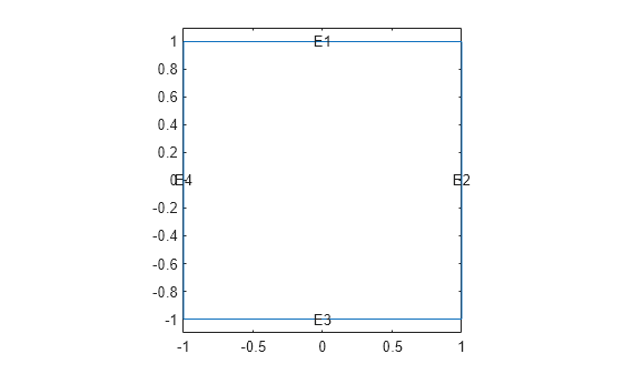
model = createpde;
geometryFromEdges(model,@squareg);
pdegplot(model,'EdgeLabels','on')
ylim([-1.1,1.1])
axis equal

Figure contains an axes object. The axes object contains 5 objects of type line, text.

Set Dirichlet boundary conditions $u = 0$ for $x = \pm 1$ , and Neumann boundary conditions

$\nabla u \cdot n = 0$

for $y = \pm 1$ . (The Neumann boundary condition is the default condition, so the second specification is redundant.)

applyBoundaryCondition(model,'dirichlet','Edge',[2,4],'u',0);
applyBoundaryCondition(model,'neumann','Edge',[1,3],'g',0);

Set the initial conditions.

u0 = 'atan(cos(pi/2*x))';
ut0 = '3*sin(pi*x).*exp(cos(pi*y))';

Set the solution times.

tlist = linspace(0,5,31);

Give coefficients for the problem.

c = 1;
a = 0;
f = 0;
d = 1;

Generate a mesh and solve the PDE.

generateMesh(model,'GeometricOrder','linear','Hmax',0.1);
u1 = hyperbolic(u0,ut0,tlist,model,c,a,f,d);

456 successful steps
51 failed attempts
1016 function evaluations
1 partial derivatives
134 LU decompositions
1015 solutions of linear systems

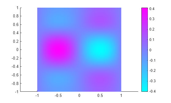
Plot the solution at the first and last times.

figure
pdeplot(model,'XYData',u1(:,1))
axis equal

Figure contains an axes object. The axes object contains an object of type patch.

figure
pdeplot(model,'XYData',u1(:,end))
axis equal

Figure contains an axes object. The axes object contains an object of type patch.

For a version of this example with animation, see Wave Equation on Square Domain.

Hyperbolic Equation Using Legacy Syntax

Open Live Script

Solve the wave equation

$\frac{\partial^{2} u}{\partial t^{2}} = Δ u$

on the square domain specified by squareg, using a geometry function to specify the geometry, a boundary function to specify the boundary conditions, and using initmesh to create the finite element mesh.

Specify the geometry as @squareg and plot the geometry.

g = @squareg;
pdegplot(g,'EdgeLabels','on')
ylim([-1.1,1.1])
axis equal

Figure contains an axes object. The axes object contains 5 objects of type line, text.

Set Dirichlet boundary conditions $u = 0$ for $x = \pm 1$ , and Neumann boundary conditions

$\nabla u \cdot n = 0$

for $y = \pm 1$ . (The Neumann boundary condition is the default condition, so the second specification is redundant.)

The squareb3 function specifies these boundary conditions.

b = @squareb3;

Set the initial conditions.

u0 = 'atan(cos(pi/2*x))';
ut0 = '3*sin(pi*x).*exp(cos(pi*y))';

Set the solution times.

tlist = linspace(0,5,31);

Give coefficients for the problem.

c = 1;
a = 0;
f = 0;
d = 1;

Create a mesh and solve the PDE.

[p,e,t] = initmesh(g);
u = hyperbolic(u0,ut0,tlist,b,p,e,t,c,a,f,d);

462 successful steps
70 failed attempts
1066 function evaluations
1 partial derivatives
156 LU decompositions
1065 solutions of linear systems

Plot the solution at the first and last times.

figure
pdeplot(p,e,t,'XYData',u(:,1))
axis equal

Figure contains an axes object. The axes object contains an object of type patch.

figure
pdeplot(p,e,t,'XYData',u(:,end))
axis equal

Figure contains an axes object. The axes object contains an object of type patch.

For a version of this example with animation, see Wave Equation on Square Domain.

Hyperbolic Solution Using Finite Element Matrices

Open Live Script

Solve a hyperbolic problem using finite element matrices.

Create a model and import the BracketWithHole.stl geometry.

model = createpde();
importGeometry(model,'BracketWithHole.stl');
figure
pdegplot(model,'FaceLabels','on')
view(30,30)
title('Bracket with Face Labels')

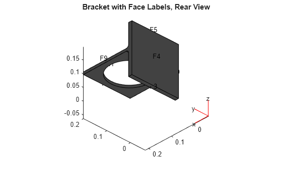
Figure contains an axes object. The axes object with title Bracket with Face Labels contains 6 objects of type quiver, text, patch, line.

figure
pdegplot(model,'FaceLabels','on')
view(-134,-32)
title('Bracket with Face Labels, Rear View')

Figure contains an axes object. The axes object with title Bracket with Face Labels, Rear View contains 6 objects of type quiver, text, patch, line.

Set coefficients c = 1, a = 0, f = 0.5, and d = 1.

c = 1;
a = 0;
f = 0.5;
d = 1;

Generate a mesh for the model.

generateMesh(model);

Create initial conditions and boundary conditions. The boundary condition for the rear face is Dirichlet with value 0. All other faces have the default boundary condition. The initial condition is u(0) = 0, du/dt(0) = x/2. Give the initial condition on the derivative by calculating the x-position of each node in xpts, and passing x/2.

applyBoundaryCondition(model,'Face',4,'u',0);
u0 = 0;
xpts = model.Mesh.Nodes(1,:);
ut0 = xpts(:)/2;

Create the associated finite element matrices.

[Kc,Fc,B,ud] = assempde(model,c,a,f);
[~,M,~] = assema(model,0,d,f);

Solve the PDE for times from 0 to 2.

tlist = linspace(0,5,50);
u = hyperbolic(u0,ut0,tlist,Kc,Fc,B,ud,M);

1487 successful steps
68 failed attempts
3015 function evaluations
1 partial derivatives
269 LU decompositions
3014 solutions of linear systems

View the solution at a few times. Scale all the plots to have the same color range by using the clim command.

umax = max(max(u));
umin = min(min(u));

subplot(2,2,1)
pdeplot3D(model,'ColorMapData',u(:,5))
clim([umin umax])
title('Time 1/2')
subplot(2,2,2)
pdeplot3D(model,'ColorMapData',u(:,10))
clim([umin umax])
title('Time 1')
subplot(2,2,3)
pdeplot3D(model,'ColorMapData',u(:,15))
clim([umin umax])
title('Time 3/2')
subplot(2,2,4)
pdeplot3D(model,'ColorMapData',u(:,20))
clim([umin umax])
title('Time 2')

Figure contains 4 axes objects. Hidden axes object 1 with title Time 1/2 contains 5 objects of type patch, quiver, text. Hidden axes object 2 with title Time 1 contains 5 objects of type patch, quiver, text. Hidden axes object 3 with title Time 3/2 contains 5 objects of type patch, quiver, text. Hidden axes object 4 with title Time 2 contains 5 objects of type patch, quiver, text.

The solution seems to have a frequency of one, because the plots at times 1/2 and 3/2 show maximum values, and those at times 1 and 2 show minimum values.

Hyperbolic Equation with Damping

Open Live Script

Solve a hyperbolic problem that includes damping. You must use the finite element matrix form to use damping.

Create a model and import the BracketWithHole.stl geometry.

model = createpde();
importGeometry(model,'BracketWithHole.stl');
figure
pdegplot(model,'FaceLabels','on')
view(30,30)
title('Bracket with Face Labels')

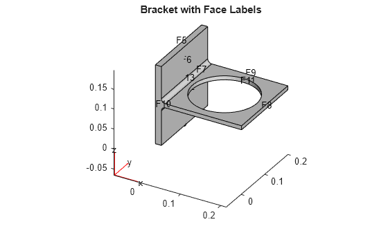
Figure contains an axes object. The axes object with title Bracket with Face Labels contains 6 objects of type quiver, text, patch, line.

figure
pdegplot(model,'FaceLabels','on')
view(-134,-32)
title('Bracket with Face Labels, Rear View')

Figure contains an axes object. The axes object with title Bracket with Face Labels, Rear View contains 6 objects of type quiver, text, patch, line.

Set coefficients c = 1, a = 0, f = 0.5, and d = 1.

c = 1;
a = 0;
f = 0.5;
d = 1;

Generate a mesh for the model.

generateMesh(model);

applyBoundaryCondition(model,'Face',4,'u',0);
u0 = 0;
xpts = model.Mesh.Nodes(1,:);
ut0 = xpts(:)/2;

Create the associated finite element matrices.

[Kc,Fc,B,ud] = assempde(model,c,a,f);
[~,M,~] = assema(model,0,d,f);

Use a damping matrix that is 10% of the mass matrix.

Damping = 0.1*M;

Solve the PDE for times from 0 to 2.

tlist = linspace(0,5,50);
u = hyperbolic(u0,ut0,tlist,Kc,Fc,B,ud,M,'DampingMatrix',Damping);

1434 successful steps
67 failed attempts
2771 function evaluations
1 partial derivatives
279 LU decompositions
2770 solutions of linear systems

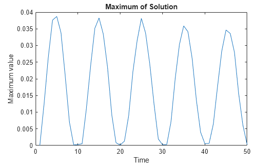
Plot the maximum value at each time. The oscillations damp slightly as time increases.

plot(max(u))
xlabel('Time')
ylabel('Maximum value')
title('Maximum of Solution')

Figure contains an axes object. The axes object with title Maximum of Solution, xlabel Time, ylabel Maximum value contains an object of type line.

Input Arguments

collapse all

`u0` — Initial condition
vector | character vector | character array | string scalar | string vector

Initial condition, specified as a scalar, vector of nodal values, character vector, character array, string scalar, or string vector. The initial condition is the value of the solution u at the initial time, specified as a column vector of values at the nodes. The nodes are either p in the [p,e,t] data structure, or are model.Mesh.Nodes.

If the initial condition is a constant scalar v, specify u0 as v.
If there are Np nodes in the mesh, and N equations in the system of PDEs, specify u0 as a column vector of Np*N elements, where the first Np elements correspond to the first component of the solution u, the second Np elements correspond to the second component of the solution u, etc.
Give a text expression of a function, such as 'x.^2 + 5*cos(x.*y)'. If you have a system of N > 1 equations, give a text array such as
```
char('x.^2 + 5*cos(x.*y)',...
    'tanh(x.*y)./(1+z.^2)')
```

Example: x.^2+5*cos(y.*x)

Data Types: double | char | string
Complex Number Support: Yes

`ut0` — Initial derivative
vector | character vector | character array | string scalar | string vector

Initial derivative, specified as a vector, character vector, character array, string scalar, or string vector. The initial gradient is the value of the derivative of the solution u at the initial time, specified as a vector of values at the nodes. The nodes are either p in the [p,e,t] data structure, or are model.Mesh.Nodes.

If the initial derivative is a constant value v, specify u0 as v.
If there are Np nodes in the mesh, and N equations in the system of PDEs, specify ut0 as a vector of Np*N elements, where the first Np elements correspond to the first component of the solution u, the second Np elements correspond to the second component of the solution u, etc.
Give a text expression of a function, such as 'x.^2 + 5*cos(x.*y)'. If you have a system of N > 1 equations, use a text array such as
```
char('x.^2 + 5*cos(x.*y)',...
    'tanh(x.*y)./(1+z.^2)')
```

Example: p(1,:).^2+5*cos(p(2,:).*p(1,:))

Data Types: double | char | string
Complex Number Support: Yes

`tlist` — Solution times
real vector

Solution times, specified as a real vector. The solver returns the solution to the PDE at the solution times.

Example: 0:0.2:4

Data Types: double

`model` — PDE model
`PDEModel` object

PDE model, specified as a PDEModel object.

Example: model = createpde

`c` — PDE coefficient
scalar | matrix | character vector | character array | string scalar | string vector | coefficient function

PDE coefficient, specified as a scalar, matrix, character vector, character array, string scalar, string vector, or coefficient function. c represents the c coefficient in the scalar PDE

$d \frac{\partial^{2} u}{\partial t^{2}} - \nabla \cdot (c \nabla u) + a u = f$

or in the system of PDEs

$d \frac{\partial^{2} u}{\partial t^{2}} - \nabla \cdot (c \otimes \nabla u) + a u = f$

Example: 'cosh(x+y.^2)'

Data Types: double | char | string | function_handle
Complex Number Support: Yes

`a` — PDE coefficient
scalar | matrix | character vector | character array | string scalar | string vector | coefficient function

PDE coefficient, specified as a scalar, matrix, character vector, character array, string scalar, string vector, or coefficient function. a represents the a coefficient in the scalar PDE

$d \frac{\partial^{2} u}{\partial t^{2}} - \nabla \cdot (c \nabla u) + a u = f$

or in the system of PDEs

$d \frac{\partial^{2} u}{\partial t^{2}} - \nabla \cdot (c \otimes \nabla u) + a u = f$

Example: 2*eye(3)

Data Types: double | char | string | function_handle
Complex Number Support: Yes

`f` — PDE coefficient
scalar | matrix | character vector | character array | string scalar | string vector | coefficient function

PDE coefficient, specified as a scalar, matrix, character vector, character array, string scalar, string vector, or coefficient function. f represents the f coefficient in the scalar PDE

$d \frac{\partial^{2} u}{\partial t^{2}} - \nabla \cdot (c \nabla u) + a u = f$

or in the system of PDEs

$d \frac{\partial^{2} u}{\partial t^{2}} - \nabla \cdot (c \otimes \nabla u) + a u = f$

Example: char('sin(x)';'cos(y)';'tan(z)')

Data Types: double | char | string | function_handle
Complex Number Support: Yes

`d` — PDE coefficient
scalar | matrix | character vector | character array | string scalar | string vector | coefficient function

PDE coefficient, specified as a scalar, matrix, character vector, character array, string scalar, string vector, or coefficient function. d represents the d coefficient in the scalar PDE

$d \frac{\partial^{2} u}{\partial t^{2}} - \nabla \cdot (c \nabla u) + a u = f$

or in the system of PDEs

$d \frac{\partial^{2} u}{\partial t^{2}} - \nabla \cdot (c \otimes \nabla u) + a u = f$

Example: 2*eye(3)

Data Types: double | char | string | function_handle
Complex Number Support: Yes

`b` — Boundary conditions
boundary matrix | boundary file

Boundary conditions, specified as a boundary matrix or boundary file. Pass a boundary file as a function handle or as a file name. A boundary matrix is generally an export from the PDE Modeler app.

Example: b = 'circleb1', b = "circleb1", or b = @circleb1

Data Types: double | char | string | function_handle

`p` — Mesh points
matrix

Mesh points, specified as a 2-by-Np matrix of points, where Np is the number of points in the mesh. For a description of the (p,e,t) matrices, see Mesh Data as [p,e,t] Triples.

Typically, you use the p, e, and t data exported from the PDE Modeler app, or generated by initmesh or refinemesh.

Example: [p,e,t] = initmesh(gd)

Data Types: double

`e` — Mesh edges
matrix

Mesh edges, specified as a 7-by-Ne matrix of edges, where Ne is the number of edges in the mesh. For a description of the (p,e,t) matrices, see Mesh Data as [p,e,t] Triples.

Typically, you use the p, e, and t data exported from the PDE Modeler app, or generated by initmesh or refinemesh.

Example: [p,e,t] = initmesh(gd)

Data Types: double

`t` — Mesh triangles
matrix

Mesh triangles, specified as a 4-by-Nt matrix of triangles, where Nt is the number of triangles in the mesh. For a description of the (p,e,t) matrices, see Mesh Data as [p,e,t] Triples.

Typically, you use the p, e, and t data exported from the PDE Modeler app, or generated by initmesh or refinemesh.

Example: [p,e,t] = initmesh(gd)

Data Types: double

`Kc` — Stiffness matrix
sparse matrix | full matrix

Stiffness matrix, specified as a sparse matrix or as a full matrix. See Elliptic Equations. Typically, Kc is the output of assempde.

`Fc` — Load vector
vector

Load vector, specified as a vector. See Elliptic Equations. Typically, Fc is the output of assempde.

`B` — Dirichlet nullspace
sparse matrix

Dirichlet nullspace, returned as a sparse matrix. See Algorithms. Typically, B is the output of assempde.

`ud` — Dirichlet vector
vector

Dirichlet vector, returned as a vector. See Algorithms. Typically, ud is the output of assempde.

`M` — Mass matrix
sparse matrix | full matrix

Mass matrix. specified as a sparse matrix or a full matrix. See Elliptic Equations.

To obtain the input matrices for pdeeig, hyperbolic or parabolic, run both assema and assempde:

[Kc,Fc,B,ud] = assempde(model,c,a,f);
[~,M,~] = assema(model,0,d,f);

Note

Create the M matrix using assema with d, not a, as the argument before f.

Data Types: double
Complex Number Support: Yes

`rtol` — Relative tolerance for ODE solver
`1e-3` (default) | positive real

Relative tolerance for ODE solver, specified as a positive real.

Example: 2e-4

Data Types: double

`atol` — Absolute tolerance for ODE solver
`1e-6` (default) | positive real

Absolute tolerance for ODE solver, specified as a positive real.

Example: 2e-7

Data Types: double

`D` — Damping matrix
matrix

Damping matrix, specified as a matrix. D has the same size as the stiffness matrix Kc or the mass matrix M. When you include D, hyperbolic solves the following ODE for the variable v:

$B^{T} M B \frac{d^{2} v}{d t^{2}} + B^{T} D B \frac{d v}{d t} + K v = F$

with initial condition u0 and initial derivative ut0. Then hyperbolic returns the solution u = B*v + ud.

For an example using D, see Dynamics of Damped Cantilever Beam.

Example: alpha*M + beta*K

Data Types: double
Complex Number Support: Yes

Output Arguments

collapse all

`u` — PDE solution
matrix

PDE solution, returned as a matrix. The matrix is Np*N-by-T, where Np is the number of nodes in the mesh, N is the number of equations in the PDE (N = 1 for a scalar PDE), and T is the number of solution times, meaning the length of tlist. The solution matrix has the following structure.

The first Np elements of each column in u represent the solution of equation 1, then next Np elements represent the solution of equation 2, etc. The solution u is the value at the corresponding node in the mesh.
Column i of u represents the solution at time tlist(i).

To obtain the solution at an arbitrary point in the geometry, use pdeInterpolant.

Algorithms

collapse all

Hyperbolic Equations

Partial Differential Equation Toolbox™ solves equations of the form

$m \frac{\partial^{2} u}{\partial t^{2}} + d \frac{\partial u}{\partial t} - \nabla \cdot (c \nabla u) + a u = f$

When the d coefficient is 0, but m is not, the documentation calls this a hyperbolic equation, whether or not it is mathematically of the hyperbolic form.

Using the same ideas as for the parabolic equation, hyperbolic implements the numerical solution of

$m \frac{\partial^{2} u}{\partial t^{2}} - \nabla \cdot (c \nabla u) + a u = f$

for x in Ω, where x represents a 2-D or 3-D point, with the initial conditions

$\begin{matrix} u (x, 0) = u_{0} (x) \\ \frac{\partial u}{\partial t} (x, 0) = v_{0} (x) \end{matrix}$

for all x in Ω, and usual boundary conditions. In particular, solutions of the equation u_tt - cΔu = 0 are waves moving with speed $\sqrt{c}$ .

Using a given mesh of Ω, the method of lines yields the second order ODE system

$M \frac{d^{2} U}{d t^{2}} + K U = F$

with the initial conditions

$\begin{matrix} U_{i} (0) = u_{0} (x_{i}) \forall i \\ \frac{d}{d t} U_{i} (0) = v_{0} (x_{i}) \forall i \end{matrix}$

after we eliminate the unknowns fixed by Dirichlet boundary conditions. As before, the stiffness matrix K and the mass matrix M are assembled with the aid of the function assempde from the problems

–∇ · (c∇u) + au = f and –∇ · (0∇u) + mu = 0.

(1)

hyperbolic internally calls assema, assemb, and assempde to create finite element matrices corresponding to the problem. It calls ode15s to solve the resulting system of ordinary differential equations.

Finite Element Basis for 3-D

The finite element method for 3-D geometry is similar to the 2-D method described in Elliptic Equations. The main difference is that the elements in 3-D geometry are tetrahedra, which means that the basis functions are different from those in 2-D geometry.

It is convenient to map a tetrahedron to a canonical tetrahedron with a local coordinate system (r,s,t).

Tetrahedral mesh element with the corner nodes p1, p2, p3, and p4 in the coordinate system with the r, s, t axes. The node p1 is located at the origin.

In local coordinates, the point p1 is at (0,0,0), p2 is at (1,0,0), p3 is at (0,1,0), and p4 is at (0,0,1).

For a linear tetrahedron, the basis functions are

$\begin{matrix} ϕ_{1} = 1 - r - s - t \\ ϕ_{2} = r \\ ϕ_{3} = s \\ ϕ_{4} = t \end{matrix}$

For a quadratic tetrahedron, there are additional nodes at the edge midpoints.

Tetrahedral mesh element with the additional nodes p5, p6, p7, p8, p9, and p10 at the edge midpoints

The corresponding basis functions are

$\begin{matrix} ϕ_{1} = 2 {(1 - r - s - t)}^{2} - (1 - r - s - t) \\ ϕ_{2} = 2 r^{2} - r \\ ϕ_{3} = 2 s^{2} - s \\ ϕ_{4} = 2 t^{2} - t \\ ϕ_{5} = 4 r (1 - r - s - t) \\ ϕ_{6} = 4 r s \\ ϕ_{7} = 4 s (1 - r - s - t) \\ ϕ_{8} = 4 t (1 - r - s - t) \\ ϕ_{9} = 4 r t \\ ϕ_{10} = 4 s t \end{matrix}$

As in the 2-D case, a 3-D basis function ϕ_i takes the value 0 at all nodes j, except for node i, where it takes the value 1.

Systems of PDEs

Partial Differential Equation Toolbox software can also handle systems of N partial differential equations over the domain Ω. We have the elliptic system

$- \nabla \cdot (c \otimes \nabla u) + a u = f$

the parabolic system

$d \frac{\partial u}{\partial t} - \nabla \cdot (c \otimes \nabla u) + a u = f$

the hyperbolic system

$d \frac{\partial^{2} u}{\partial t^{2}} - \nabla \cdot (c \otimes \nabla u) + a u = f$

and the eigenvalue system

$- \nabla \cdot (c \otimes \nabla u) + a u = λ d u$

where c is an N-by-N-by-D-by-D tensor, and D is the geometry dimensions, 2 or 3.

For 2-D systems, the notation $\nabla \cdot (c \otimes \nabla u)$ represents an N-by-1 matrix with an (i,1)-component

$\sum_{j = 1}^{N} (\frac{\partial}{\partial x} c_{i, j, 1, 1} \frac{\partial}{\partial x} + \frac{\partial}{\partial x} c_{i, j, 1, 2} \frac{\partial}{\partial y} + \frac{\partial}{\partial y} c_{i, j, 2, 1} \frac{\partial}{\partial x} + \frac{\partial}{\partial y} c_{i, j, 2, 2} \frac{\partial}{\partial y}) u_{j}$

For 3-D systems, the notation $\nabla \cdot (c \otimes \nabla u)$ represents an N-by-1 matrix with an (i,1)-component

$\begin{array}{l} \sum_{j = 1}^{N} (\frac{\partial}{\partial x} c_{i, j, 1, 1} \frac{\partial}{\partial x} + \frac{\partial}{\partial x} c_{i, j, 1, 2} \frac{\partial}{\partial y} + \frac{\partial}{\partial x} c_{i, j, 1, 3} \frac{\partial}{\partial z}) u_{j} \\ + \sum_{j = 1}^{N} (\frac{\partial}{\partial y} c_{i, j, 2, 1} \frac{\partial}{\partial x} + \frac{\partial}{\partial y} c_{i, j, 2, 2} \frac{\partial}{\partial y} + \frac{\partial}{\partial y} c_{i, j, 2, 3} \frac{\partial}{\partial z}) u_{j} \\ + \sum_{j = 1}^{N} (\frac{\partial}{\partial z} c_{i, j, 3, 1} \frac{\partial}{\partial x} + \frac{\partial}{\partial z} c_{i, j, 3, 2} \frac{\partial}{\partial y} + \frac{\partial}{\partial z} c_{i, j, 3, 3} \frac{\partial}{\partial z}) u_{j} \end{array}$

The symbols a and d denote N-by-N matrices, and f denotes a column vector of length N.

The elements c_ijkl, a_ij, d_ij, and f_i of c, a, d, and f are stored row-wise in the MATLAB^® matrices c, a, d, and f. The case of identity, diagonal, and symmetric matrices are handled as special cases. For the tensor c_ijkl this applies both to the indices i and j, and to the indices k and l.

Partial Differential Equation Toolbox software does not check the ellipticity of the problem, and it is quite possible to define a system that is not elliptic in the mathematical sense. The preceding procedure that describes the scalar case is applied to each component of the system, yielding a symmetric positive definite system of equations whenever the differential system possesses these characteristics.

The boundary conditions now in general are mixed, i.e., for each point on the boundary a combination of Dirichlet and generalized Neumann conditions,

$\begin{array}{l} h u = r \\ n \cdot (c \otimes \nabla u) + q u = g + h^{'} μ \end{array}$

For 2-D systems, the notation $n \cdot (c \otimes \nabla u)$ represents an N-by-1 matrix with (i,1)-component

$\sum_{j = 1}^{N} (\cos (α) c_{i, j, 1, 1} \frac{\partial}{\partial x} + \cos (α) c_{i, j, 1, 2} \frac{\partial}{\partial y} + \sin (α) c_{i, j, 2, 1} \frac{\partial}{\partial x} + \sin (α) c_{i, j, 2, 2} \frac{\partial}{\partial y}) u_{j}$

where the outward normal vector of the boundary is $n = (\cos (α), \sin (α))$ .

For 3-D systems, the notation $n \cdot (c \otimes \nabla u)$ represents an N-by-1 matrix with (i,1)-component

$\begin{array}{l} \sum_{j = 1}^{N} (\cos (α) c_{i, j, 1, 1} \frac{\partial}{\partial x} + \cos (α) c_{i, j, 1, 2} \frac{\partial}{\partial y} + \cos (α) c_{i, j, 1, 3} \frac{\partial}{\partial z}) u_{j} \\ + \sum_{j = 1}^{N} (\cos (β) c_{i, j, 2, 1} \frac{\partial}{\partial x} + \cos (β) c_{i, j, 2, 2} \frac{\partial}{\partial y} + \cos (β) c_{i, j, 2, 3} \frac{\partial}{\partial z}) u_{j} \\ + \sum_{j = 1}^{N} (\cos (γ) c_{i, j, 3, 1} \frac{\partial}{\partial x} + \cos (γ) c_{i, j, 3, 2} \frac{\partial}{\partial y} + \cos (γ) c_{i, j, 3, 3} \frac{\partial}{\partial z}) u_{j} \end{array}$

where the outward normal to the boundary is

$n = (\cos (α), \cos (β), \cos (γ))$

There are M Dirichlet conditions and the h-matrix is M-by-N, M ≥ 0. The generalized Neumann condition contains a source $h^{'} μ$ , where the Lagrange multipliers μ are computed such that the Dirichlet conditions become satisfied. In a structural mechanics problem, this term is exactly the reaction force necessary to satisfy the kinematic constraints described by the Dirichlet conditions.

The rest of this section details the treatment of the Dirichlet conditions and may be skipped on a first reading.

Partial Differential Equation Toolbox software supports two implementations of Dirichlet conditions. The simplest is the “Stiff Spring” model, so named for its interpretation in solid mechanics. See Elliptic Equations for the scalar case, which is equivalent to a diagonal h-matrix. For the general case, Dirichlet conditions

hu = r

are approximated by adding a term

$L (h^{'} h u - h^{'} r)$

to the equations KU = F, where L is a large number such as 10⁴ times a representative size of the elements of K.

When this number is increased, hu = r will be more accurately satisfied, but the potential ill-conditioning of the modified equations will become more serious.

The second method is also applicable to general mixed conditions with nondiagonal h, and is free of the ill-conditioning, but is more involved computationally. Assume that there are N_p nodes in the mesh. Then the number of unknowns is N_pN = N_u. When Dirichlet boundary conditions fix some of the unknowns, the linear system can be correspondingly reduced. This is easily done by removing rows and columns when u values are given, but here we must treat the case when some linear combinations of the components of u are given, hu = r. These are collected into HU = R where H is an M-by-N_u matrix and R is an M-vector.

With the reaction force term the system becomes

KU +H´ µ = F

HU = R.

The constraints can be solved for M of the U-variables, the remaining called V, an N_u – M vector. The null space of H is spanned by the columns of B, and U = BV + u_d makes U satisfy the Dirichlet conditions. A permutation to block-diagonal form exploits the sparsity of H to speed up the following computation to find B in a numerically stable way. µ can be eliminated by pre-multiplying by B´ since, by the construction, HB = 0 or B´H´ = 0. The reduced system becomes

B´ KBV = B´ F – B´Ku_d

which is symmetric and positive definite if K is.

Version History

Introduced before R2006a

expand all

R2016a: Not recommended

hyperbolic is not recommended. Use solvepde instead. There are no plans to remove hyperbolic.

R2012b: Coefficients of hyperbolic PDEs as functions of the solution and its gradient

You can now solve hyperbolic equations whose coefficients depend on the solution u or on the gradient of u.

hyperbolic

Syntax

Description

Examples

Hyperbolic Equation

Hyperbolic Equation Using Legacy Syntax

Hyperbolic Solution Using Finite Element Matrices

Hyperbolic Equation with Damping

Input Arguments

u0 — Initial condition vector | character vector | character array | string scalar | string vector

ut0 — Initial derivative vector | character vector | character array | string scalar | string vector

tlist — Solution times real vector

model — PDE model PDEModel object

c — PDE coefficient scalar | matrix | character vector | character array | string scalar | string vector | coefficient function

a — PDE coefficient scalar | matrix | character vector | character array | string scalar | string vector | coefficient function

f — PDE coefficient scalar | matrix | character vector | character array | string scalar | string vector | coefficient function

d — PDE coefficient scalar | matrix | character vector | character array | string scalar | string vector | coefficient function

b — Boundary conditions boundary matrix | boundary file

p — Mesh points matrix

e — Mesh edges matrix

t — Mesh triangles matrix

Kc — Stiffness matrix sparse matrix | full matrix

Fc — Load vector vector

B — Dirichlet nullspace sparse matrix

ud — Dirichlet vector vector

M — Mass matrix sparse matrix | full matrix

rtol — Relative tolerance for ODE solver 1e-3 (default) | positive real

atol — Absolute tolerance for ODE solver 1e-6 (default) | positive real

D — Damping matrix matrix

Output Arguments

u — PDE solution matrix

Algorithms

Hyperbolic Equations

Finite Element Basis for 3-D

Systems of PDEs

Version History

R2016a: Not recommended

R2012b: Coefficients of hyperbolic PDEs as functions of the solution and its gradient

See Also

`u0` — Initial condition
vector | character vector | character array | string scalar | string vector

`ut0` — Initial derivative
vector | character vector | character array | string scalar | string vector

`tlist` — Solution times
real vector

`model` — PDE model
`PDEModel` object

`c` — PDE coefficient
scalar | matrix | character vector | character array | string scalar | string vector | coefficient function

`a` — PDE coefficient
scalar | matrix | character vector | character array | string scalar | string vector | coefficient function

`f` — PDE coefficient
scalar | matrix | character vector | character array | string scalar | string vector | coefficient function

`d` — PDE coefficient
scalar | matrix | character vector | character array | string scalar | string vector | coefficient function

`b` — Boundary conditions
boundary matrix | boundary file

`p` — Mesh points
matrix

`e` — Mesh edges
matrix

`t` — Mesh triangles
matrix

`Kc` — Stiffness matrix
sparse matrix | full matrix

`Fc` — Load vector
vector

`B` — Dirichlet nullspace
sparse matrix

`ud` — Dirichlet vector
vector

`M` — Mass matrix
sparse matrix | full matrix

`rtol` — Relative tolerance for ODE solver
`1e-3` (default) | positive real

`atol` — Absolute tolerance for ODE solver
`1e-6` (default) | positive real

`D` — Damping matrix
matrix

`u` — PDE solution
matrix