Main Content

setInitialConditions

Give initial conditions or initial solution

Description

setInitialConditions(model,u0) sets initial conditions in model. Use this syntax for stationary nonlinear problems or time-dependent problems where the time derivative is first order.

Note

Include geometry in model before using setInitialConditions.

example

setInitialConditions(model,u0,ut0) use this syntax for time-dependent problems where a time derivative is second order, such as a hyperbolic problem.

example

setInitialConditions(___,RegionType,RegionID) sets initial conditions on a geometry region using any of the arguments in the previous syntaxes.

example

setInitialConditions(model,results) sets the initial guess for stationary nonlinear problems using the solution results from a previous analysis on the same geometry and mesh. The initial derivative for stationary problems is 0.

example

setInitialConditions(model,results,iT) sets the initial conditions for time-dependent problems using the solution results corresponding to the solution time index iT. If you do not specify the time index iT, setInitialConditions uses the last solution time in results.

example

ic = setInitialConditions(___) returns a handle to the initial conditions object.

Examples

collapse all

Create a PDE model, import geometry, and set the initial condition to 50 on the entire geometry.

model = createpde();
importGeometry(model,"BracketWithHole.stl");
setInitialConditions(model,50);

Set different initial conditions for each component of a system of PDEs.

Create a PDE model for a system with five components. Import the Block.stl geometry.

model = createpde(5);
importGeometry(model,"Block.stl");

Set the initial conditions for each component to twice the component number.

u0 = [2:2:10]';
setInitialConditions(model,u0)
ans = 
  GeometricInitialConditions with properties:

           RegionType: 'cell'
             RegionID: 1
         InitialValue: [5x1 double]
    InitialDerivative: []

Set different initial conditions on each portion of the L-shaped membrane geometry.

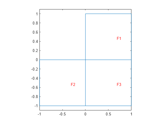
Create a model, set the geometry function, and view the subdomain labels.

model = createpde();
geometryFromEdges(model,@lshapeg);
pdegplot(model,"FaceLabels","on")
axis equal
ylim([-1.1,1.1])

Figure contains an axes object. The axes object contains 4 objects of type line, text.

Set subdomain 1 to initial value -1, subdomain 2 to initial value 1, and subdomain 3 to initial value 5.

setInitialConditions(model,-1);
setInitialConditions(model,1,"Face",2);
setInitialConditions(model,5,"Face",3);

The initial setting applies to the entire geometry. The subsequent settings override the initial settings for regions 2 and 3.

Set initial conditions for the L-shaped membrane geometry to be x2+y2, except in the lower left square where it is x2-y4.

model = createpde();
geometryFromEdges(model,@lshapeg);
pdegplot(model,"FaceLabels","on")
axis equal
ylim([-1.1,1.1])

Figure contains an axes object. The axes object contains 4 objects of type line, text.

Set the initial conditions to x2+y2.

initfun = @(location)location.x.^2 + location.y.^2;
setInitialConditions(model,initfun);

Set the initial conditions on region 2 to x2-y4. This setting overrides the first setting because you apply it after the first setting.

initfun2 = @(location)location.x.^2 - location.y.^4;
setInitialConditions(model,initfun2,"Face",2);

Hyperbolic equations have nonzero m coefficient, so you must set both the u0 and ut0 arguments.

Import the Block.stl to a PDE model with N = 3 components.

model = createpde(3);
importGeometry(model,"Block.stl");

Set the initial condition value to be 0 for all components. Set the initial derivative.

ut0=[4+xx2+y2+z25-tanh(z)10yx2+y2+z2]

To create this initial gradient, write a function file, and ensure that the function is on your MATLAB path.

function ut0 = ut0fun(location)

M = length(location.x);

ut0 = zeros(3,M);

denom = location.x.^2+location.y.^2+location.z.^2;

ut0(1,:) = 4 + location.x./denom;

ut0(2,:) = 5 - tanh(location.z);

ut0(3,:) = 10*location.y./denom;

end

Set the initial conditions.

setInitialConditions(model,0,@ut0fun)
ans = 
  GeometricInitialConditions with properties:

           RegionType: 'cell'
             RegionID: 1
         InitialValue: 0
    InitialDerivative: @ut0fun

Set initial conditions using the solution from a previous analysis on the same geometry and mesh.

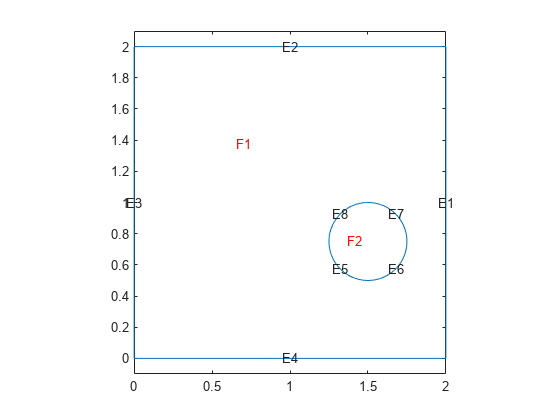
Create and view the geometry: a square with a circular subdomain.

% Square centered at (1,1), circle centered at (1.5,0.5).
rect1 = [3;4;0;2;2;0;0;0;2;2];
circ1 = [1;1.5;.75;0.25];
% Append extra zeros to the circle;
circ1 = [circ1;zeros(length(rect1)-length(circ1),1)];
gd = [rect1,circ1];
ns = char('rect1','circ1');
ns = ns';
sf = 'rect1+circ1';
[dl,bt] = decsg(gd,sf,ns);
pdegplot(dl,"EdgeLabels","on","FaceLabels","on")
axis equal
ylim([-0.1,2.1])

Figure contains an axes object. The axes object contains 11 objects of type line, text.

Include the geometry in a PDE model, set boundary and initial conditions, and specify coefficients.

model = createpde();
geometryFromEdges(model,dl);

% Set boundary conditions that the upper
% and left edges are at temperature 10.
applyBoundaryCondition(model,"dirichlet", ...
                             "Edge",[2,3],"u",10);

% Set initial conditions that the square region
% is at temperature 0,
% and the circle is at temperature 100.
setInitialConditions(model,0);
setInitialConditions(model,100,"Face",2);

specifyCoefficients(model,"m",0,...
                          "d",1,...
                          "c",1,...
                          "a",0,...
                          "f",0);

Solve the problem for times 0 through 1/2 in steps of 0.01.

generateMesh(model,"Hmax",0.05);
tlist = 0:0.01:0.5;
results = solvepde(model,tlist);

Plot the solution for times 0.02, 0.04, 0.1, and 0.5.

sol = results.NodalSolution;

subplot(2,2,1)
pdeplot(model,"XYData",sol(:,3))
title("Time 0.02")
subplot(2,2,2)
pdeplot(model,"XYData",sol(:,5))
title("Time 0.04")
subplot(2,2,3)
pdeplot(model,"XYData",sol(:,11))
title("Time 0.1")
subplot(2,2,4)
pdeplot(model,"XYData",sol(:,51))
title("Time 0.5")

Figure contains 4 axes objects. Axes object 1 with title Time 0.02 contains an object of type patch. Axes object 2 with title Time 0.04 contains an object of type patch. Axes object 3 with title Time 0.1 contains an object of type patch. Axes object 4 with title Time 0.5 contains an object of type patch.

Now, resume the analysis and solve the problem for times from 1/2 to 1. Use the previously obtained solution for time 1/2 as an initial condition. Since 1/2 is the last element in tlist, you do not need to specify the solution time index. By default, setInitialConditions uses the last solution index.

setInitialConditions(model,results)
ans = 
  NodalInitialConditions with properties:

         InitialValue: [7385x1 double]
    InitialDerivative: []

Solve the problem for times 1/2 through 1 in steps of 0.01.

tlist1 = 0.5:0.01:1.0;
results1 = solvepde(model,tlist1);

Plot the solution for times 0.5, 0.7, 0.9, and 1.

sol1 = results1.NodalSolution;

figure

subplot(2,2,1)
pdeplot(model,"XYData",sol1(:,1))
title("Time 0.5")
subplot(2,2,2)
pdeplot(model,"XYData",sol1(:,21))
title("Time 0.7")
subplot(2,2,3)
pdeplot(model,"XYData",sol1(:,41))
title("Time 0.9")
subplot(2,2,4)
pdeplot(model,"XYData",sol1(:,51))
title("Time 1.0")

Figure contains 4 axes objects. Axes object 1 with title Time 0.5 contains an object of type patch. Axes object 2 with title Time 0.7 contains an object of type patch. Axes object 3 with title Time 0.9 contains an object of type patch. Axes object 4 with title Time 1.0 contains an object of type patch.

To use the previously obtained solution for a particular solution time instead of the last one, specify the solution time index as a third parameter of setInitialConditions. For example, use the solution at time 0.2, which is the 21st element in tlist.

setInitialConditions(model,results,21)
ans = 
  NodalInitialConditions with properties:

         InitialValue: [7385x1 double]
    InitialDerivative: []

Solve the problem for times 0.2 through 1 in steps of 0.01.

tlist2 = 0.2:0.01:1.0;
results2 = solvepde(model,tlist2);

Input Arguments

collapse all

PDE model, specified as a PDEModel object.

Example: model = createpde

Initial conditions, specified as a scalar, a column vector of length N, or a function handle. N is the size of the system of PDEs. See Equations You Can Solve Using Partial Differential Equation Toolbox.

  • Scalar — Use it to represent a constant initial value for all solution components throughout the domain.

  • Column vector — Use it to represent a constant initial value for each of the N solution components throughout the domain.

  • Function handle — Use it to represent the initial conditions as a function of position. The function must be of the form

    u0 = initfun(location)

    Solvers pass location as a structure with fields location.x, location.y, and, for 3-D problems, location.z. initfun must return a matrix u0 of size N-by-M, where M = length(location.x).

Example: setInitialConditions(model,10)

Data Types: double | function_handle
Complex Number Support: Yes

Initial condition for time derivative, specified as a scalar, a column vector of length N, or a function handle. N is the size of the system of PDEs. See Equations You Can Solve Using Partial Differential Equation Toolbox. You must specify ut0 when there is a nonzero second-order time-derivative coefficient m.

  • Scalar — Use it to represent a constant initial value for all solution components throughout the domain.

  • Column vector — Use it to represent a constant initial value for each of the N solution components throughout the domain.

  • Function handle — Use it to represent the initial conditions as a function of position. The function must be of the form

    u0 = initfun(location)

    Solvers pass location as a structure with fields location.x, location.y, and, for 3-D problems, location.z. initfun must return a matrix u0 of size N-by-M, where M = length(location.x).

Example: setInitialConditions(model,10,@initfun)

Data Types: double | function_handle
Complex Number Support: Yes

Geometric region type, specified as "Face", "Edge", "Vertex", or "Cell".

When there are multiple initial condition assignments, solvers use the following precedence rules for determining the initial condition.

  • If there are multiple assignments to the same geometric region, solvers use the last applied setting.

  • If there are separate assignments to a geometric region and the boundaries of that region, the solvers use the specified assignment on the region and choose the assignment on the boundary as follows. The solvers give an "Edge" assignment precedence over a "Face" assignment, even if you specify a "Face" assignment after an "Edge" assignment. The precedence levels are "Vertex (highest precedence), "Edge", "Face", "Cell" (lowest precedence).

  • If there is an assignment made with the results object, solvers use that assignment instead of all previous assignments.

Example: setInitialConditions(model,10,"Face",1:4)

Data Types: char | string

Geometric region ID, specified as a vector of positive integers. Find the region IDs by using pdegplot.

Example: setInitialConditions(model,10,"Face",1:4)

Data Types: double

PDE solution, specified as a StationaryResults object or a TimeDependentResults object. Create results using solvepde or createPDEResults.

Example: results = solvepde(model)

Time index, specified as a positive integer.

Example: setInitialConditions(model,results,21)

Data Types: double

Output Arguments

collapse all

Handle to initial condition, returned as an object. ic associates the initial condition with the geometric region in the case of a geometric assignment or the nodes in the case of a results-based assignment.

Tips

  • To ensure that the model has the correct TimeDependent property setting, if possible specify coefficients before setting initial conditions.

  • To avoid assigning initial conditions to a wrong region, ensure that you are using the correct geometric region IDs by plotting and visually inspecting the geometry.

Version History

Introduced in R2016a

expand all