pdenonlin
(Not recommended) Solve nonlinear elliptic PDE problem
pdenonlin is not recommended. Use solvepde
instead.
Syntax
Description
u = pdenonlin(model,c,a,f)
with geometry, boundary conditions, and finite element
mesh in model, and coefficients
c, a, and
f. In this context,
“nonlinear” means some coefficient in
c, a, or
f depends on the solution
u or its gradient. If the PDE
is a system of equations
(model.PDESystemSize > 1),
then pdenonlin solves the
system of equations
u = pdenonlin(___,Name,Value)Name,
Value pairs.
Examples
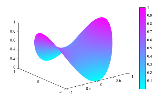
Solve a minimal surface problem. Because this problem has a nonlinear c coefficient, use pdenonlin to solve it.
Create a model and include circular geometry using the built-in circleg function.
model = createpde;
geometryFromEdges(model,@circleg);
Set the coefficients.
a = 0;
f = 0;
c = '1./sqrt(1+ux.^2+uy.^2)';
Set a Dirichlet boundary condition with value .
boundaryfun = @(region,state)region.x.^2;
applyBoundaryCondition(model,'edge',1:model.Geometry.NumEdges,...
                      'u',boundaryfun,'Vectorized','on');
Generate a mesh and solve the problem.
generateMesh(model,'GeometricOrder','linear','Hmax',0.1);
u = pdenonlin(model,c,a,f);
pdeplot(model,'XYData',u,'ZData',u)
Solve the minimal surface problem using the legacy approach for creating boundary conditions and geometry.
Create the geometry using the built-in circleg function. Plot the geometry to see the edge labels.
g = @circleg;
pdegplot(g,'EdgeLabels','on')
axis equal
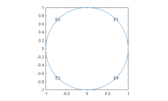
Create Dirichlet boundary conditions with value .Create the following file and save it on your MATLAB® path.
function [qmatrix,gmatrix,hmatrix,rmatrix] = pdex2bound(p,e,u,time)
ne = size(e,2); % number of edges
qmatrix = zeros(1,ne);
gmatrix = qmatrix;
hmatrix = zeros(1,2*ne);
rmatrix = hmatrix;
for k = 1:ne
    x1 = p(1,e(1,k)); % x at first point in segment
    x2 = p(1,e(2,k)); % x at second point in segment
    xm = (x1 + x2)/2; % x at segment midpoint
    y1 = p(2,e(1,k)); % y at first point in segment
    y2 = p(2,e(2,k)); % y at second point in segment
    ym = (y1 + y2)/2; % y at segment midpoint
    switch e(5,k)
        case {1,2,3,4}
            hmatrix(k) = 1;
            hmatrix(k+ne) = 1;
            rmatrix(k) = x1^2;
            rmatrix(k+ne) = x2^2;
    end
end
Set the coefficients and boundary conditions.
a = 0;
f = 0;
c = '1./sqrt(1+ux.^2+uy.^2)';
b = @pdex2bound;
Generate a mesh and solve the problem.
[p,e,t] = initmesh(g,'Hmax',0.1);
u = pdenonlin(b,p,e,t,c,a,f);
pdeplot(p,e,t,'XYData',u,'ZData',u)

Solve a nonlinear 3-D problem with nontrivial geometry.
Import the geometry from the BracketWithHole.stl file. Plot the geometry and face labels.
model = createpde();
importGeometry(model,'BracketWithHole.stl');
figure
pdegplot(model,'FaceLabels','on','FaceAlpha',0.5)
view(30,30)
title('Bracket with Face Labels')
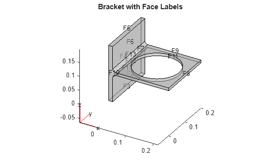
figure
pdegplot(model,'FaceLabels','on','FaceAlpha',0.5)
view(-134,-32)
title('Bracket with Face Labels, Rear View')
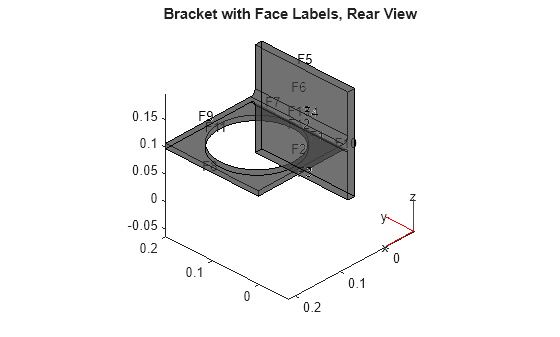
Set a Dirichlet boundary condition with value 1000 on the back face, which is face 4. Set the large faces 1 and 7, and also the circular face 11, to have Neumann boundary conditions with value g = -10. Do not set boundary conditions on the other faces. Those faces default to Neumann boundary conditions with value g = 0.
applyBoundaryCondition(model,'Face',4,'u',1000);
applyBoundaryCondition(model,'Face',[1,7,11],'g',-10);
Set the c coefficient to 1, f to 0.1, and a to the nonlinear value '0.1 + 0.001*u.^2'.
c = 1;
f = 0.1;
a = '0.1 + 0.001*u.^2';
Generate the mesh and solve the PDE. Start from the initial guess u0 = 1000, which matches the value you set on face 4. Turn on the Report option to observe the convergence during the solution.
generateMesh(model);
u = pdenonlin(model,c,a,f,'U0',1000,'Report','on');
Iteration     Residual     Step size  Jacobian: full
   0          7.0647e-01
   1          1.0526e-01   1.0000000
   2          3.1239e-02   1.0000000
   3          8.7260e-03   1.0000000
   4          1.7663e-03   1.0000000
   5          1.3894e-04   1.0000000
   6          1.0998e-06   1.0000000
Plot the solution on the geometry boundary.
pdeplot3D(model,'ColorMapData',u)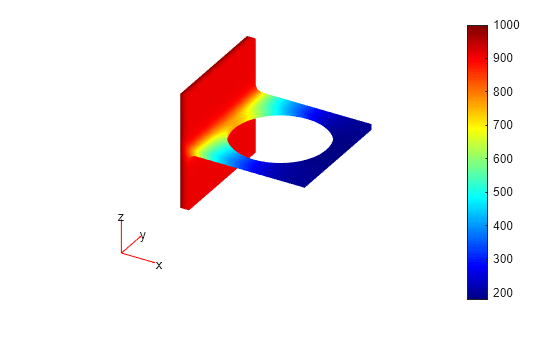
Input Arguments
Name-Value Arguments
Output Arguments
Tips
If the Newton iteration does not converge,
pdenonlindisplays the error messageToo many iterationsorStepsize too small.If the initial guess produces matrices containing
NaNorInfelements,pdenonlindisplays the error messageUnsuitable initial guess U0 (default: U0 = 0).If you have very small coefficients, or very small geometric dimensions,
pdenonlincan fail to converge, or can converge to an incorrect solution. If so, you can sometimes obtain better results by scaling the coefficients or geometry dimensions to be of order one.