Remaining Useful Life Estimation Using Convolutional Neural Network

Download Data Set

This example uses the Turbofan Engine Degradation Simulation data set [1]. The data set is in ZIP file format, and contains run-to-failure time-series data for four different sets (namely FD001, FD002, FD003, and FD004) simulated under different combinations of operational conditions and fault modes.

This example uses only the FD001 data set, which is further divided into training and test subsets. The training subset contains simulated time series data for 100 engines. Each engine has several sensors whose values are recorded at a given instance in a continuous process. Hence, the sequence of recorded data varies in length and corresponds to a full run-to-failure (RTF) instance. The test subset contains 100 partial sequences and corresponding values of the remaining useful life at the end of each sequence.

Create a directory to store the Turbofan Engine Degradation Simulation data set.

dataFolder = "data";
if ~exist(dataFolder,'dir')
    mkdir(dataFolder);
end

Download and extract the Turbofan Engine Degradation Simulation data set.

filename = matlab.internal.examples.downloadSupportFile("nnet","data/TurbofanEngineDegradationSimulationData.zip");
unzip(filename,dataFolder)

The data folder now contains text files with 26 columns of numbers, separated by spaces. Each row is a snapshot of data taken during a single operational cycle, and each column represents a different variable:

Preprocess Training Data

Load the data using the function localLoadData. The function extracts the data from a data file and returns a table which contains the training predictors and corresponding response (i.e., RUL) sequences. Each row represents a different engine.

filenameTrainPredictors = fullfile(dataFolder,"train_FD001.txt");
rawTrain = localLoadData(filenameTrainPredictors);

Examine the run-to-failure data for one of the engines.

head(rawTrain.X{1},8)

    id    timeStamp    op_setting_1    op_setting_2    op_setting_3    sensor_1    sensor_2    sensor_3    sensor_4    sensor_5    sensor_6    sensor_7    sensor_8    sensor_9    sensor_10    sensor_11    sensor_12    sensor_13    sensor_14    sensor_15    sensor_16    sensor_17    sensor_18    sensor_19    sensor_20    sensor_21
    __    _________    ____________    ____________    ____________    ________    ________    ________    ________    ________    ________    ________    ________    ________    _________    _________    _________    _________    _________    _________    _________    _________    _________    _________    _________    _________

    1         1          -0.0007         -0.0004           100          518.67      641.82      1589.7      1400.6      14.62       21.61       554.36      2388.1      9046.2        1.3         47.47       521.66         2388       8138.6       8.4195        0.03          392         2388          100         39.06       23.419  
    1         2           0.0019         -0.0003           100          518.67      642.15      1591.8      1403.1      14.62       21.61       553.75        2388      9044.1        1.3         47.49       522.28       2388.1       8131.5       8.4318        0.03          392         2388          100            39       23.424  
    1         3          -0.0043          0.0003           100          518.67      642.35        1588      1404.2      14.62       21.61       554.26      2388.1      9052.9        1.3         47.27       522.42         2388       8133.2       8.4178        0.03          390         2388          100         38.95       23.344  
    1         4           0.0007               0           100          518.67      642.35      1582.8      1401.9      14.62       21.61       554.45      2388.1      9049.5        1.3         47.13       522.86       2388.1       8133.8       8.3682        0.03          392         2388          100         38.88       23.374  
    1         5          -0.0019         -0.0002           100          518.67      642.37      1582.8      1406.2      14.62       21.61          554      2388.1      9055.1        1.3         47.28       522.19         2388       8133.8       8.4294        0.03          393         2388          100          38.9       23.404  
    1         6          -0.0043         -0.0001           100          518.67       642.1      1584.5      1398.4      14.62       21.61       554.67        2388      9049.7        1.3         47.16       521.68         2388       8132.9       8.4108        0.03          391         2388          100         38.98       23.367  
    1         7            0.001          0.0001           100          518.67      642.48      1592.3      1397.8      14.62       21.61       554.34        2388      9059.1        1.3         47.36       522.32         2388       8132.3       8.3974        0.03          392         2388          100          39.1       23.377  
    1         8          -0.0034          0.0003           100          518.67      642.56        1583        1401      14.62       21.61       553.85        2388      9040.8        1.3         47.24       522.47         2388       8131.1       8.4076        0.03          391         2388          100         38.97       23.311  

Examine the response data for one of the engines.

rawTrain.Y{1}(1:8)

ans = 8×1

   191
   190
   189
   188
   187
   186
   185
   184

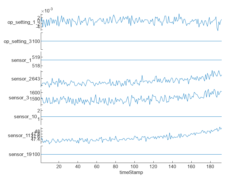
Visualize the time-series data for some of the predictors.

stackedplot(rawTrain.X{1},[3,5,6,7,8,15,16,24],XVariable='timeStamp')

Remove Features with Less Variability

Features that remain constant for all time steps can negatively impact the training. Use the prognosability function to measure the variability of features at failure.

prog = prognosability(rawTrain.X,"timeStamp");

For some features, prognosability is equal to zero or NaN. Discard these features.

idxToRemove = prog.Variables==0 | isnan(prog.Variables);
featToRetain = prog.Properties.VariableNames(~idxToRemove);
for i = 1:height(rawTrain)
    rawTrain.X{i} = rawTrain.X{i}{:,featToRetain};
end

Normalize Training Predictors

Normalize the training predictors to have zero mean and unit variance.

[~,Xmu,Xsigma] = zscore(vertcat(rawTrain.X{:}));
preTrain = table();
for i = 1:numel(rawTrain.X)
    preTrain.X{i} = (rawTrain.X{i} - Xmu) ./ Xsigma;
end

Clip Responses

The response data represents the RUL value over life for each engine and is based individual engine lifetime. The sequence assumes a linear degradation from the time of the initial measurement to the time of engine failure.

In order for network to focus on the part of the data where engines are more likely to fail (end of the engine's life), clip the responses at the threshold of 150. Clipping the responses causes the network to treat instances with higher RUL values as equal.

rulThreshold = 150;
for i = 1:numel(rawTrain.Y)
    preTrain.Y{i} = min(rawTrain.Y{i},rulThreshold);
end

This figure shows the first observation and the corresponding response (RUL), which is clipped at the threshold. The green overlay defines the clipping region on both sensor amd RUL plots.

Prepare Data for Padding

This network supports input data with varying sequence lengths. When passing data through the network, the software pads, truncates, or splits sequences so that all the sequences in each mini-batch have the specified length.

To minimize the amount of padding added to the mini-batches, sort the training data by sequence length. Then, choose a mini-batch size which divides the training data evenly and reduces the amount of padding in the mini-batches.

Sort the training data by sequence length.

for i = 1:size(preTrain,1)
    preTrain.X{i} = preTrain.X{i}';    %Transpose training data to have features in the first dimension
    preTrain.Y{i} = preTrain.Y{i}';    %Transpose responses corresponding to the training data
    sequence = preTrain.X{i};
    sequenceLengths(i) = size(sequence,2); 
end

[sequenceLengths,idx] = sort(sequenceLengths,'descend');
XTrain = preTrain.X(idx);
YTrain = preTrain.Y(idx);

Network Architecture

The deep convolutional neural network architecture used for RUL estimation is described in [1].

Here, you process and sort the data in a sequence format, with the first dimension representing the number of selected features and the second dimension representing the length of the time sequence. You bundle convolutional layers with batch normalization layer followed by an activation layer (relu in this case) and then stack the layers together for feature extraction. The fully connected layers are used at the end to get the final RUL value as output.

The selected network architecture applies a 1-D convolution along the time sequence direction only. Therefore, the order of features does not impact the training and only trends in one feature at a time are considered.

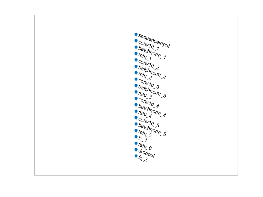
Define the network architecture. Create a CNN that consists of five consecutive sets of a convolution 1-d, batch normalization and, a relu layer, with increasing filterSize and numFilters as the first two input arguments to convolution1dLayer, followed by a fully connected layer of size numHiddenUnits and a dropout layer with a dropout probability of 0.5. Since the network predicts the remaining useful life (RUL) of the turbofan engine, set numResponses to 1 in the second fully connected layer.

To compensate for the varying time-sequences in the training data, use Padding="causal" as the Name-value pair input argument in convolution1dLayer.

numFeatures = size(XTrain{1},1);
numHiddenUnits = 100;
numResponses = 1;

layers = [
    sequenceInputLayer(numFeatures)
    convolution1dLayer(5,32,Padding="causal")
    batchNormalizationLayer
    reluLayer()
    convolution1dLayer(7,64,Padding="causal")
    batchNormalizationLayer
    reluLayer()
    convolution1dLayer(11,128,Padding="causal")
    batchNormalizationLayer
    reluLayer()
    convolution1dLayer(13,256,Padding="causal")
    batchNormalizationLayer
    reluLayer()
    convolution1dLayer(15,512,Padding="causal")
    batchNormalizationLayer
    reluLayer()
    fullyConnectedLayer(numHiddenUnits)
    reluLayer()
    dropoutLayer(0.5)
    fullyConnectedLayer(numResponses)];

Train Network

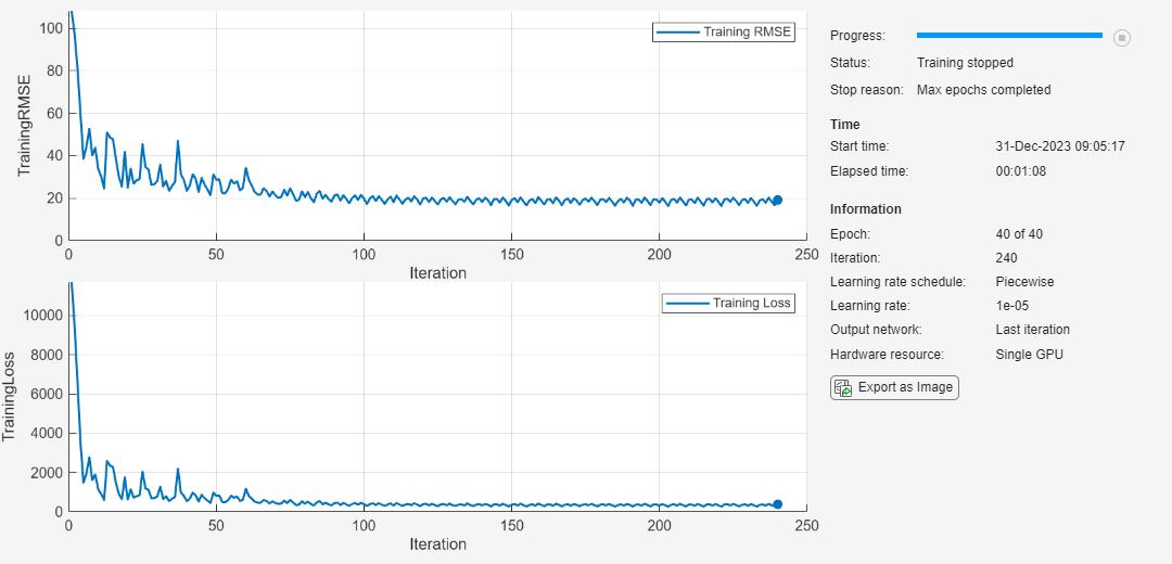
Specify trainingOptions (Deep Learning Toolbox). Train for 40 epochs with minibatches of size 16 using the Adam optimizer. Set LearnRateSchedule to piecewise. Specify the learning rate as 0.01. To prevent the gradients from exploding, set the gradient threshold to 1. To keep the sequences sorted by length, set 'Shuffle' to 'never'. Turn on the training progress plot and also set the Metrics to 'rmse' to view the RMSE plot. Set the InputDataFormats as CTB because the training data contains features in the first dimension, time-series sequence in the second dimension, and the batches of the data in the third dimension. Turn off the command window output (Verbose).

maxEpochs = 40;
miniBatchSize = 16;

options = trainingOptions('adam',...
    LearnRateSchedule='piecewise',...
    MaxEpochs=maxEpochs,...
    MiniBatchSize=miniBatchSize,...
    InitialLearnRate=0.01,...
    GradientThreshold=1,...
    Shuffle='never',...
    Plots='training-progress',...
    Metrics='rmse',...
    InputDataFormats='CTB',...
    Verbose=0);

Train the network using trainnet and specify the loss function as mean squared error (mse). This should take about 1-2 minutes.

net = trainnet(XTrain,YTrain,layers,"mse",options);

Plot the layer graph of the network to visualize the underlying network architecture.

figure;
plot(net)

Test Network

The test data contains 100 partial sequences and corresponding values of the remaining useful life at the end of each sequence.

filenameTestPredictors = fullfile(dataFolder,'test_FD001.txt');
filenameTestResponses = fullfile(dataFolder,'RUL_FD001.txt');
dataTest = localLoadData(filenameTestPredictors,filenameTestResponses);

Prepare the test data set for predictions by performing the same preprocessing steps you use to prepare the training data set.

for i = 1:numel(dataTest.X)
    dataTest.X{i} = dataTest.X{i}{:,featToRetain};
    dataTest.X{i} = (dataTest.X{i} - Xmu) ./ Xsigma;
    dataTest.Y{i} = min(dataTest.Y{i},rulThreshold);
end

Create a table for storing the predicted response (YPred) along with the true response (Y). Make predictions on the test data using minibatchpredict. To prevent the function from adding padding to the test data, specify the mini-batch size as 1 to get RUL value for each observation in the test data. Set InputDataFormats as CTB because the test data is also in the same format as the training data.

predictions = table(Size=[height(dataTest) 2],VariableTypes=["cell","cell"],VariableNames=["Y","YPred"]);

for i=1:height(dataTest)
    unit = dataTest.X{i}';   
    predictions.Y{i} = dataTest.Y{i}';
    predictions.YPred{i} = minibatchpredict(net,unit,MiniBatchSize=1,InputDataFormats='CTB');
end

Performance Metrics

Compute the root mean squared error (RMSE) across all time cycles of the test sequences to analyze how well the network performs on the test data.

for i = 1:size(predictions,1)
    predictions.RMSE(i) = sqrt(mean((predictions.Y{i} - predictions.YPred{i}).^2));
end

Create a histogram to visualize the distribution of RMSE values across all test engines.

figure;
histogram(predictions.RMSE,NumBins=10);
title("RMSE ( Mean: " + round(mean(predictions.RMSE),2) + " , StDev: " + round(std(predictions.RMSE),2) + " )");
ylabel('Frequency');
xlabel('RMSE');

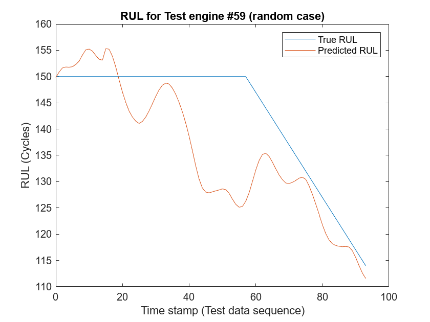
Additionally, to see how the network predictor performs throughout the given sequence of data in the test engines, use the localLambdaPlot function to plot the predicted RUL against the true RUL of a random test engine.

figure;
localLambdaPlot(predictions,"random");

The result shows that the CNN deep learning architecture for estimating RUL of the turbo engine data is a viable approach to predict RUL. The RMSE values at all timestamps indicates that the network can perform well towards the end of the given test sequence data. Therefore, having a brief history of the sensor data is important when trying to predict RUL.

Helper Functions

Load Data Function

This function loads run-to-failure data from the provided text file and groups time-series data and its corresponding RUL values in a table as predictors and responses.

function data = localLoadData(filenamePredictors,varargin)

if isempty(varargin)
    filenameResponses = []; 
else
    filenameResponses = varargin{:};
end

%% Load the text file as a table
rawData = readtable(filenamePredictors);

% Add variable names to the table
VarNames = {...
    'id', 'timeStamp', 'op_setting_1', 'op_setting_2', 'op_setting_3', ...
    'sensor_1', 'sensor_2', 'sensor_3', 'sensor_4', 'sensor_5', ...
    'sensor_6', 'sensor_7', 'sensor_8', 'sensor_9', 'sensor_10', ...
    'sensor_11', 'sensor_12', 'sensor_13', 'sensor_14', 'sensor_15', ...
    'sensor_16', 'sensor_17', 'sensor_18', 'sensor_19', 'sensor_20', ...
    'sensor_21'};
rawData.Properties.VariableNames = VarNames;

if ~isempty(filenameResponses)
    RULTest = readmatrix(filenameResponses);
end

% Split the signals for each unit ID
IDs = rawData{:,1};
nID = unique(IDs);
numObservations = numel(nID);

% Initialize a table for storing data
data = table(Size=[numObservations 2],...
    VariableTypes={'cell','cell'},...
    VariableNames={'X','Y'});

for i=1:numObservations
    idx = IDs == nID(i);
    data.X{i} = rawData(idx,:);
    if isempty(filenameResponses)
        % Calculate RUL from time column for train data
        data.Y{i} = flipud(rawData.timeStamp(idx))-1;
    else
        % Use RUL values from filenameResponses for test data
        sequenceLength = sum(idx);
        endRUL = RULTest(i);
        data.Y{i} = [endRUL+sequenceLength-1:-1:endRUL]'; %#ok<NBRAK> 
    end
end
end

Lambda Plot function

This helper function accepts the predictions table and a lambdaCase argument, and plots the predicted RUL against the true RUL throughout its sequence (at every timestamp) for a visualization of how the prediction changes with every timestamp. The second argument, lambdaCase, can be the test engine number or one of a set of valid strings to find an engine number : "random", "best", "worst", or "average".

function localLambdaPlot(predictions,lambdaCase)

if isnumeric(lambdaCase)
    idx = lambdaCase;
else
    switch lambdaCase
        case {"Random","random","r"}
            idx = randperm(height(predictions),1); % Randomly choose a test case to plot
        case {"Best","best","b"}
            idx = find(predictions.RMSE == min(predictions.RMSE)); % Best case
        case {"Worst","worst","w"}
            idx = find(predictions.RMSE == max(predictions.RMSE)); % Worst case
        case {"Average","average","a"}
            err = abs(predictions.RMSE-mean(predictions.RMSE));
            idx = find(err==min(err),1);
    end
end
y = predictions.Y{idx};
yPred = predictions.YPred{idx};
x = 0:numel(y)-1;
plot(x,y,x,yPred)
legend("True RUL","Predicted RUL")
xlabel("Time stamp (Test data sequence)")
ylabel("RUL (Cycles)")

title("RUL for Test engine #"+idx+ " ("+lambdaCase+" case)")
end

References