rcstruncone
Radar cross section of truncated cone
Syntax
Description
rcspat = rcstruncone(r1,r2,height,c,fc)r1 is the
radius of the small end of the cone, r2 is the radius of the large end,
and height is the cone height. The radar cross section is a function of
signal frequency, fc, and signal propagation speed,
c. You can create a non-truncated cone by setting
r1 to zero. The cone points downward towards the
xy-plane. The origin is located at the apex of a the non-truncated cone
constructed by extending the truncated cone to an apex.
Examples
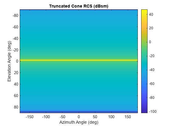
Display the radar cross section (RCS) pattern of a truncated cone as a function of azimuth angle and elevation. The truncated cone has a bottom radius of 9.0 cm and a top radius of 12.5 cm. The cone height is 1 m. The operating frequency is 4.5 GHz.
Define the truncated cone geometry and signal parameters.
c = physconst('Lightspeed');
fc = 4.5e9;
radbot = 0.090;
radtop = 0.125;
hgt = 1;
Compute the RCS for all directions using the default direction values.
[rcspat,azresp,elresp] = rcstruncone(radbot,radtop,hgt,c,fc);
imagesc(azresp,elresp,pow2db(rcspat))
xlabel('Azimuth Angle (deg)')
ylabel('Elevation Angle (deg)')
title('Truncated Cone RCS (dBsm)')
colorbar
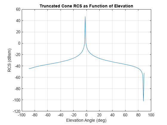
Plot the radar cross section (RCS) pattern of a truncated cone as a function of elevation for a fixed azimuth angle of 5 degrees. The cone has a bottom radius of 9.0 cm and a top radius of 12.5 cm. The truncated cone height is 1 m. The operating frequency is 4.5.
Define the truncated cone geometry and signal parameters.
c = physconst('Lightspeed');
fc = 4.5e9;
radbot = 0.090;
radtop = 0.125;
hgt = 1;
Compute the RCS at an azimuth angle of 5 degrees.
az = 5.0;
el = -90:90;
[rcspat,azresp,elresp] = rcstruncone(radbot,radtop,hgt,c,fc,az,el);
plot(elresp,pow2db(rcspat))
xlabel('Elevation Angle (deg)')
ylabel('RCS (dBsm)')
title('Truncated Cone RCS as Function of Elevation')
grid on
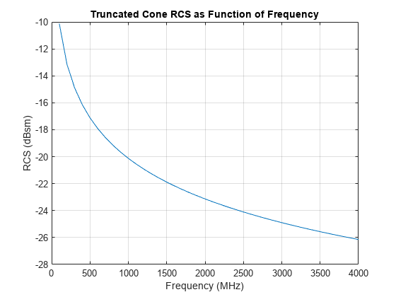
Plot the radar cross section (RCS) pattern of a truncated cone as a function of frequency for a single direction. The cone has a bottom radius of 9.0 cm and a top radius of 12.5 cm. The truncated cone height is 1 m.
Specify the truncated cone geometry and signal parameters.
c = physconst('Lightspeed');
radbot = 0.090;
radtop = 0.125;
hgt = 1;
Compute the RCS over a range of frequencies for a single direction.
az = 5.0;
el = 20.0;
fc = (100:100:4000)*1e6;
[rcspat,azpat,elpat] = rcstruncone(radbot,radtop,hgt,c,fc,az,el);
disp([azpat,elpat])
5 20
plot(fc/1e6,pow2db(squeeze(rcspat)))
xlabel('Frequency (MHz)')
ylabel('RCS (dBsm)')
title('Truncated Cone RCS as Function of Frequency')
grid on
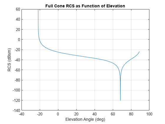
Plot the radar cross section (RCS) pattern of a full cone as a function of elevation for a fixed azimuth angle. To define a full cone set the bottom radius to zero. Set the top radius to 20.0 cm and the cone height to 50 cm. Assume the operating frequency is 4.5 GHz and the azimuth angle is 5 degrees.
Define the cone geometry and signal parameters.
c = physconst('Lightspeed');
fc = 4.5e9;
radsmall = 0.0;
radlarge = 0.20;
hgt = 0.5;
Compute the RCS for a fixed azimuth angle of 5 degrees.
az = 5.0;
el = -89:0.1:89;
[rcspat,azresp,elresp] = rcstruncone(radsmall,radlarge,hgt,c,fc,az,el);
plot(elresp,pow2db(rcspat))
xlabel('Elevation Angle (deg)')
ylabel('RCS (dBsm)')
title('Full Cone RCS as Function of Elevation')
grid on
Input Arguments
Output Arguments
More About
This section describes the convention used to define azimuth and elevation angles.
The azimuth angle of a vector is the angle between the x-axis and its orthogonal projection onto the xy-plane. The angle is positive when going from the x-axis toward the y-axis. Azimuth angles lie between –180° and 180° degrees, inclusive. The elevation angle is the angle between the vector and its orthogonal projection onto the xy-plane. The angle is positive when going toward the positive z-axis from the xy-plane. Elevation angles lie between –90° and 90° degrees, inclusive.

References
[1] Mahafza, Bassem. Radar Systems Analysis and Design Using MATLAB, 2nd Ed. Boca Raton, FL: Chapman & Hall/CRC, 2005.
Extended Capabilities
Version History
Introduced in R2021a
See Also
rcscylinder | rcsdisc | rcssphere | phased.BackscatterRadarTarget | phased.RadarTarget