Train Multiple Agents for Area Coverage

This example uses:

This example demonstrates a multi-agent collaborative task in which you train three proximal policy optimization (PPO) agents to achieve full coverage of a grid-world environment. As shown in this example, if you define your environment behavior using MATLAB code, you can also incorporate it into a Simulink® environment using MATLAB Function blocks.

Fix Random Seed Generator to Improve Reproducibility

The example code may involve computation of random numbers at various stages such as initialization of the agent, creation of the actor and critic, resetting the environment during simulations, generating observations (for stochastic environments), generating exploration actions, and sampling min-batches of experiences for learning. Fixing the random number stream preserves the sequence of the random numbers every time you run the code and improves reproducibility of results. You will fix the random number stream at various locations in the example.

Fix the random number stream with the seed 0 and random number algorithm Mersenne twister. For more information on random number generation see rng.

previousRngState = rng(0,"twister")

previousRngState = struct with fields:
     Type: 'twister'
     Seed: 0
    State: [625x1 uint32]

The output previousRngState is a structure that contains information about the previous state of the stream. You will restore the state at the end of the example.

Environment Description

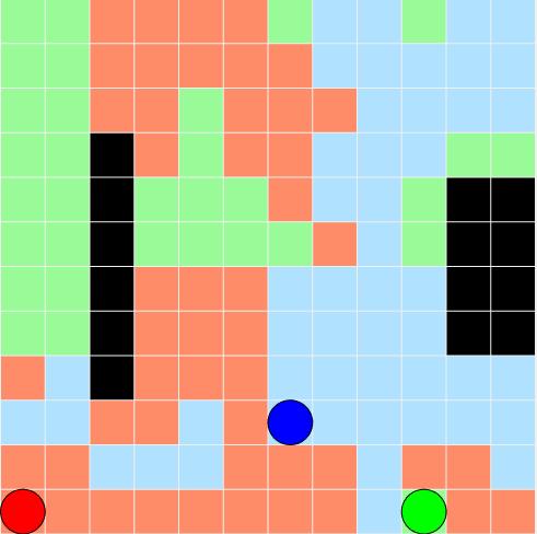
The environment in this example is a 12x12 grid world containing obstacles, with unexplored cells marked in white and obstacles marked in black. The environment contains three robots, represented by the red, green, and blue circles. Three proximal policy optimization agents with discrete action spaces control the robots. To learn more about PPO agents, see Proximal Policy Optimization (PPO) Agent.

The agents provide one of five possible movement actions (WAIT, UP, DOWN, LEFT, or RIGHT) to their respective robots. The robots decide whether an action is legal or illegal. For example, an action of moving LEFT when the robot is located next to the left boundary of the environment is deemed illegal. Similarly, actions for colliding against obstacles and other agents in the environment are illegal actions and draw penalties. The overall goal is to explore all cells within a fixed time frame.

At each time step, an agent observes the environment using a 12x12x4 image. Each of the four channels in the image captures the following information in order:

Cells with obstacles.
Current position of the robot (self) being controlled.
Position of other (friend) robots.
Cells that have been explored during the episode.

The following figure shows an example of what the agent controlling the green robot observes for a given time step.

For the grid world environment:

The search area is a 12x12 grid with obstacles.
The observation for each agent is a 12x12x4 image.
The discrete action set contains five actions (WAIT=0, UP=1, DOWN=2, LEFT=3, RIGHT=4).
The simulation terminates when the grid is fully explored or the maximum number of steps is reached.

At each time step, agents receive the following rewards:

+2 for moving to a previously unexplored cell (white).
-1 for an illegal action (attempt to move outside the boundary or collide against other robots and obstacles).
-1 for an action that results in no motion (lazy penalty).
-0.5 for moving to an explored cell.
+100 if the grid is fully explored.

Create Environment Object

Define the locations of obstacles within the grid using a matrix of indices. The first column contains the row indices, and the second column contains the column indices.

obsMat = [ ...
    4 3; ...
    5 3; ...
    6 3; ...
    7 3; ...
    8 3; ...
    9 3; ...
    5 11; ... 
    6 11; ...
    7 11; ...
    8 11; ...
    5 12; ...
    6 12; ...
    7 12; ...
    8 12 ];

Initialize the robot positions.

sA0 = [2 2];
sB0 = [11 4];
sC0 = [3 12];
s0 = [sA0; sB0; sC0];

Configure the initial condition of the grid.

% initial grid
g0 = zeros(12,12);

% obstacle cells have the value 1.0
for idx = 1:size(obsMat,1)
    r = obsMat(idx,1);
    c = obsMat(idx,2);
    g0(r,c) = 1.0;
end

% robot cells have the values:
% 0.25 (red), 
% 0.50 (green), 
% and 0.75 (blue)
g0(sA0(1),sA0(2)) = 0.25;
g0(sB0(1),sB0(2)) = 0.50;
g0(sC0(1),sC0(2)) = 0.75;

Specify the sample time, simulation time, and maximum number of steps per episode.

Ts = 0.1;
Tf = 100;
maxsteps = ceil(Tf/Ts);

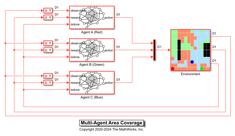
Open the model. There are three RL Agent blocks and a subsystem block that models the area coverage environment.

mdl = "rlAreaCoverage";
open_system(mdl)

The environment dynamics is implemented using MATLAB Function blocks. Navigate to the Environment subsystem to view the implementation.

For a related example on how to call environment functions from Simulink, see Create and Simulate Same Environment in Both MATLAB and Simulink.

open_system(mdl+"/Environment")

Note that the states of the environment (grid, numSteps, numExplored and nextX signals) are updated iteratively in the feedback loop. Initial values for those signals are specified in the unit delay blocks to ensure the environment is correctly initialized.

In this example, the agents are homogeneous and have the same observation and action specifications. Create the observation and action specifications for the environment. For more information, see rlNumericSpec and rlFiniteSetSpec.

% Define observation specifications.
obsSize = [12 12 4];
oinfo = rlNumericSpec(obsSize);
oinfo.Name = "observations";

% Define action specifications.
numAct = 5;
actionSpace = {0,1,2,3,4};
ainfo = rlFiniteSetSpec(actionSpace);
ainfo.Name = "actions";

Specify the block paths for the agents.

blks = mdl + ... 
    ["/Agent A (Red)","/Agent B (Green)","/Agent C (Blue)"];

Create the environment object, specifying the same observation and action specifications for all three agents.

obsInfos = {oinfo,oinfo,oinfo};
actInfos = {ainfo,ainfo,ainfo};
env = rlSimulinkEnv(mdl,blks,obsInfos,actInfos);

Specify a reset function for the environment. The function resetMap (provided at the end of this example) ensures that the robots start from random initial positions at the beginning of each episode. The random initialization makes the agents robust to different starting positions and can improve training performance.

env.ResetFcn = @(in) resetMap(in, obsMat);

Create PPO Agents With Custom Networks

The PPO agents in this example operate on a discrete action space and rely on actor and critic functions to learn the optimal policies. The agents maintain deep neural network-based function approximators for the actors and critics with similar network structures (a combination of convolution and fully connected layers). The critic outputs a scalar value representing the state value $V (s)$ . The actor outputs the probabilities $π (a | s)$ of taking each of the five actions WAIT, UP, DOWN, LEFT, or RIGHT.

Create the actor and critic functions using the following steps.

Create the actor and critic deep neural networks.
Create the actor function objects using the rlDiscreteCategoricalActor command.
Create the critic function objects using the rlValueFunction command.

When you create the agent networks, the initial parameters are initialized with random values. Fix the random number stream so that the agent is always initialized with the same parameter values.

rng(0,"twister");

Use the same network structure for all three agents.

actorNetwork = [
    imageInputLayer(obsSize)
    convolution2dLayer(3,16,Padding="same", ...
    PaddingValue=-1,Stride=2)
    reluLayer
    maxPooling2dLayer(3,Padding="same",Stride=2)
    fullyConnectedLayer(256)
    reluLayer
    fullyConnectedLayer(256)
    reluLayer
    fullyConnectedLayer(numAct)
    softmaxLayer
    ];
actorNetwork = dlnetwork(actorNetwork);

criticNetwork = [
    imageInputLayer(obsSize)
    convolution2dLayer(3,16,Padding="same", ...
    PaddingValue=-1,Stride=2)
    reluLayer
    maxPooling2dLayer(3,Padding="same",Stride=2)
    fullyConnectedLayer(256)
    reluLayer
    fullyConnectedLayer(256)
    reluLayer
    fullyConnectedLayer(1)
    ];
criticNetwork = dlnetwork(criticNetwork);

View the summary of the actor and critic networks.

summary(actorNetwork)

   Initialized: true

   Number of learnables: 104.7k

   Inputs:
      1   'imageinput'   12x12x4 images

summary(criticNetwork)

   Initialized: true

   Number of learnables: 103.7k

   Inputs:
      1   'imageinput'   12x12x4 images

Plot the actor and critic networks.

plot(actorNetwork)

Figure contains an axes object. The axes object contains an object of type graphplot.

plot(criticNetwork)

Figure contains an axes object. The axes object contains an object of type graphplot.

Create the actor and critic objects.

for idx = 1:3
    actor(idx) = rlDiscreteCategoricalActor(actorNetwork,oinfo,ainfo);
    critic(idx) = rlValueFunction(criticNetwork,oinfo);
end

Specify training options for the critic and the actor using rlOptimizerOptions.

The agents learn using the learning rate 1e-3 for the actors and critics. A large learning rate causes drastic updates which may lead to divergent behaviors, while a low value may require many updates before reaching the optimal point.
Use a gradient threshold of 1.0 to clip the gradients. Clipping the gradients can improve training stability.
Use the L2 regularization factor 1e-4 to stabilize the training.

actorOpts  = rlOptimizerOptions( ...
    LearnRate=1e-3, ...
    GradientThreshold=1, ...
    L2RegularizationFactor=1e-4);
criticOpts = rlOptimizerOptions( ...
    LearnRate=1e-3, ...
    GradientThreshold=1, ...
    L2RegularizationFactor=1e-4);

Specify the agent options using rlPPOAgentOptions, include the training options for the actor and critic. Use the same options for all three agents.

For this training:

Use the experience horizon value of 500. A large experience horizon can improve the stability of the training.
Train with mini-batches of length 200. Smaller mini-batches are computationally efficient but may introduce variance in training. Contrarily, larger batch sizes can make the training stable but require higher memory.
Use the discount factor 0.9 to favor long term rewards.
Specify the sample time Ts=0.1 second for the agents.

agentOpts = rlPPOAgentOptions(...
    ActorOptimizerOptions=actorOpts,...
    CriticOptimizerOptions=criticOpts,...
    ExperienceHorizon=500,...
    MiniBatchSize=200,...
    SampleTime=Ts,...
    DiscountFactor=0.9);

Create the agents using the defined actors, critics, and agent options.

agentA = rlPPOAgent(actor(1),critic(1),agentOpts);
agentB = rlPPOAgent(actor(2),critic(2),agentOpts);
agentC = rlPPOAgent(actor(3),critic(3),agentOpts);

Alternatively, you can create the agents first, and then access their option object to modify the options using dot notation.

Train Agents

In this example, the agents are trained in centralized manner. Specify the following options for training:

Specify all agents under one agent group.
Specify the "centralized" learning strategy.
Run the training for at most 500 episodes, with each episode lasting at most maxsteps (1000) time steps.
Stop the training an agent when its average reward over 20 consecutive episodes is 200 or more.
Do not store simulation data in memory to improve performance. Alternatively, you can specify SimulationStorageType as "file" to store simulation data to disk.

trainOpts = rlMultiAgentTrainingOptions(...
    AgentGroups={[1,2,3]},...
    LearningStrategy="centralized",...
    MaxEpisodes=500,...
    MaxStepsPerEpisode=maxsteps,...
    SimulationStorageType="none",...
    ScoreAveragingWindowLength=20,...
    StopTrainingCriteria="AverageReward", ...
    StopTrainingValue=200);

For more information see rlMultiAgentTrainingOptions.

Fix the random stream for reproducibility.

rng(0,"twister");

To train the agents, specify an array of agents to the train function. The order of the agents in the array must match the order of agent block paths specified during environment creation. Doing so ensures that the agent objects are linked to the appropriate action and observation specifications in the environment.

Training is a computationally intensive process that takes several minutes to complete. To save time while running this example, load pretrained agent parameters by setting doTraining to false. To train the agent yourself, set doTraining to true.

doTraining = false;
if doTraining
    result = train([agentA,agentB,agentC],env,trainOpts);
else
    load("rlAreaCoverageAgents.mat","params");
    % The saved agents were trained in centralized manner 
    % with synchronized model parameters. 
    % Set the trained parameters on all agents.
    setLearnableParameters(agentA, params);
    setLearnableParameters(agentB, params);
    setLearnableParameters(agentC, params);
end

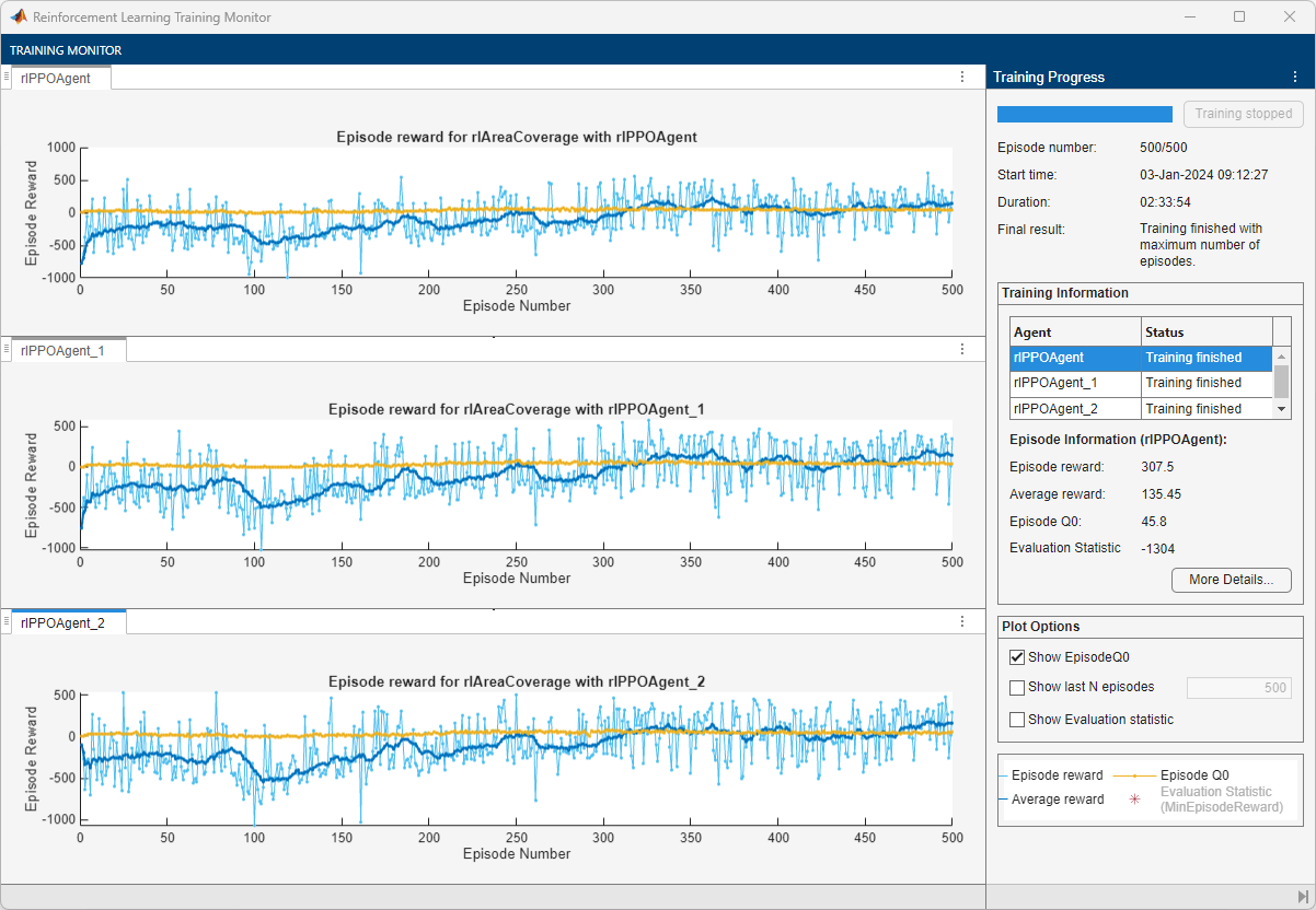
The following figure shows a snapshot of the training progress. You can expect different results due to randomness in the training process.

Simulate Agents

Fix the random stream for reproducibility.

rng(0,"twister");

Simulate the trained agents within the environment. For more information on agent simulation, see rlSimulationOptions and sim.

simOpts = rlSimulationOptions(MaxSteps=maxsteps);
experience = sim(env,[agentA,agentB,agentC],simOpts);

Figure contains an axes object. The axes object with title Steps = 264, Coverage = 100.0% contains 30 objects of type image, line, rectangle.

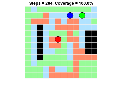
The agents are able to achieve full coverage of the grid world.

Restore the random number stream using the information stored in previousRngState.

rng(previousRngState);

Local Functions

function in = resetMap(in,obsMat)
% Reset function for multi agent area coverage example

gridSize = [12 12];
isvalid = false;
while ~isvalid
    rows = randperm(gridSize(1),3);
    cols = randperm(gridSize(2),3);
    s0 = [rows' cols'];
    if all(~all(s0(1,:) == obsMat,2)) && ...
            all(~all(s0(2,:) == obsMat,2)) && ... 
            all(~all(s0(3,:) == obsMat,2))
        isvalid = true;
    end
end

% initial grid
g0 = zeros(12,12);

% obstacle cells
for idx = 1:size(obsMat,1)
    r = obsMat(idx,1);
    c = obsMat(idx,2);
    g0(r,c) = 1.0;
end

% robot cells
g0(s0(1,1),s0(1,2)) = 0.25;
g0(s0(2,1),s0(2,2)) = 0.50;
g0(s0(3,1),s0(3,2)) = 0.75;

in = setVariable(in, 's0', s0);
in = setVariable(in, 'g0', g0);
end

Train Multiple Agents for Area Coverage

Fix Random Seed Generator to Improve Reproducibility

Environment Description

Create Environment Object

Create PPO Agents With Custom Networks

Train Agents

Simulate Agents

Local Functions

See Also

Functions

Objects

Blocks

Related Examples

More About