Create and Simulate the Same Environment in both MATLAB and Simulink

Create Environment via MATLAB Functions

To implement an environment, first, define the environment observation and action specifications. For this example, both action and observation are a simple numerical scalar.

oinfo = rlNumericSpec([1 1]);
ainfo = rlNumericSpec([1 1]);

Use the custom step and reset functions defined in the supporting files to define the behavior of a simple discrete nonlinear system. For this example, set the reward equal to the observation.

Display the step function.

type dsStepFcn.m

function [NextObs,Reward,IsDone,NextState] =  dsStepFcn(Action,State)
% Advances environment to next state and calculates outputs

NextState = 0.9*State + cos(Action);
NextObs = NextState^2;

Reward = NextObs;
IsDone = 0;

end

Note that while there is a direct feedthrough between action and next observation, there is no direct feedthrough between action and current observation. in other words, the environment is strictly causal from action to observation.

The reset function initializes the environment state to 5 and the corresponding initial observation to 25. Display the reset function.

type dsResetFcn.m

function [InitialObservation, InitialState] = dsResetFcn()
% Resets environment to an initial state

InitialState = 5;
InitialObservation = InitialState^2;

end

Use rlFunctionEnv to define a custom environment object.

menv = rlFunctionEnv(oinfo,ainfo,@dsStepFcn,@dsResetFcn);

Create Default AC Agent

Create a default actor-critic agent using the environment specifications. To ensure consistency between different simulations, prevent the agent from exploring by setting the UseExplorationPolicy option to false.

agentObj = rlACAgent(oinfo,ainfo);
agentObj.UseExplorationPolicy = false;

Simulate Agent Using MATLAB Environment

Set 6 as maximum number of simulation steps using an rlSimulationOptions object.

simopts = rlSimulationOptions(MaxSteps=6);

Then simulate the environment using sim, collecting the experience in the variable mtraj.

mtraj  = sim(menv,agentObj,simopts);

Display the action data.

mtraj.Action.act1.Data(:)'

ans = 1×6

    2.0636    1.3385    1.2263    1.1961    1.1869    1.1840

Display the observation data.

mtraj.Observation.obs1.Data(:)'

ans = 1×7

   25.0000   16.2159   14.8563   14.4907   14.3790   14.3437   14.3323

Call MATLAB Environment from Simulink using Delays on Observation and Reward

You can use a MATLAB Function (Simulink) block to call the environment step function from Simulink. As mentioned before, assume that both environment and agent have a sample time of one second.

Load the Simulink model in memory.

mdl = "dsLoopMLF3";
load_system(mdl);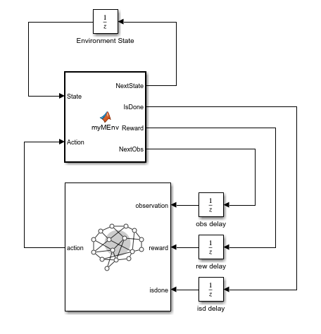

The MATLAB Function block simply calls the environment step function (the order of inputs and outputs are rearranged so that the respective signal lines do not cross each other in Simulink).

function [NextObs,IsDone,Reward,NextState] =  myMEnv(Action,State)

% Call environment step function
[NextObs,Reward,IsDone,NextState] =  dsStepFcn(Action,State);

Here, an unit delay block with an initial state set to 5 is used to store the environment state. This implementation avoids using permanent variables to implement states in the MATLAB Function block, which is subject to various limitations. For more information on such limitations, see the tables in Use Model Operating Point for Faster Simulation Workflow (Simulink) and How Stepping Through Simulation Works (Simulink).

The Simulink agent block expects the current observation as input. Therefore, use a delay block, with initial condition set to 25, to obtain the current observation. If you instead connect the agent observation port directly to the NextObs environment output, the action signal would be anticipated one step with respect to a MATLAB implementation, which would be incorrect and can also lead to an algebraic loop.

Since the reward and is-done signal received by the agent need to be synchronized with the observation signal, place delay signals also before the other two agent input ports. Here, the initial states of the reward and is-done signals are set to 25 and 0, respectively.

Create a Simulink environment from the closed loop Simulink model. First, define the agent block path within the model (the agent block uses agentObj as an agent).

blk = mdl + "/RL Agent";

Use rlSimulinkEnv to create a Simulink environment.

slenv = rlSimulinkEnv(mdl,blk,oinfo,ainfo);

Use sim to simulate the environment. Collect the experience in the variable straj.

straj = sim(slenv,agentObj,simopts);

Display the action data.

straj.Action.act1.Data(:)'

ans = 1×6

    2.0636    1.3385    1.2263    1.1961    1.1869    1.1840

Display the observation data.

straj.Observation.obs1.Data(:)'

ans = 1×7

   25.0000   16.2159   14.8563   14.4907   14.3790   14.3437   14.3323

The trajectory is identical to the one obtained from the simulation of the MATLAB environment. Note that the delays before the agent input ports prevent any algebraic loops. Also note that, using this approach, you have to initialize the delays in a way which is consistent with the initial state of the environment.

Call MATLAB Environment from Simulink using Delay on Action

You can also call the environment step function by placing a single delay on the action signal, instead of the three delays on the agent inputs. However, this strategy yields a closed loop system that generally starts from a different initial condition, and therefore generates a different trajectory.

For the first simulation or training episode, you can set the initial condition of the action delay so that the resulting trajectory is the same (just anticipated one step) as the original one. Note that this is done for this example to show that the trajectories are exactly the same, however, in general, you do not need set any specific initial condition among the feasible ones, as any trajectory would be equally valid to train or simulate the agent.

Get the initial value of the action when the observation is equal to 5^2.

a0  = getAction(agentObj,{5^2});

In the following model, the initial condition of the action delay is initialized to a0{1}.

a0{1}

ans = 2.0636

Load the Simulink model in memory.

mdl = "dsLoopMLF1";
load_system(mdl);

Define the agent block path within the model.

blk = mdl + "/RL Agent";

Use rlSimulinkEnv to create a Simulink environment.

slenv = rlSimulinkEnv(mdl,blk,oinfo,ainfo);

Use sim to simulate the environment. Collect the experience in the variable straj.

straj = sim(slenv,agentObj,simopts);

Display the action data.

straj.Action.act1.Data(:)'

ans = 1×6

    1.3385    1.2263    1.1961    1.1869    1.1840    1.1831

Display the observation data.

straj.Observation.obs1.Data(:)'

ans = 1×7

   16.2159   14.8563   14.4907   14.3790   14.3437   14.3323   14.3287

The trajectory is anticipated one step with respect to the one obtained from the simulation of the MATLAB environment.

For more information on how to deal with algebraic loops see Create Custom Simulink Environments and Algebraic Loop Concepts (Simulink).

Call Separate Environment State and Output Functions from Simulink

If you have separate state and output functions (instead of a single step function), you can call them using separate MATLAB Function (Simulink) blocks, and use a delay to represent the environment state.

Display the state function.

type dsStateFcn.m

function NextState =  dsStateFcn(Action,State)
% Advances environment to next state

NextState = 0.9*State + cos(Action);

end

Display the output function.

type dsOutputFcn.m

function [Observation,Reward,IsDone] =  dsOutputFcn(State)
% Calculates outputs

Observation = State^2;
Reward = Observation;
IsDone = 0;

end

Note that the output does not depend on the current action, since the environment is assumed to be strictly causal.

Use MATLAB Function (Simulink) blocks to call both function from Simulink, and use delays to represent the environment state. In the first Simulink model of this example, you fed the delayed NextObs signal to the observation input port of the agent block. In the following model, the corresponding signal is the delayed output function (square) of the next state signal, which is identical (from the agent perspective) to the output function of the current state signal, which is exactly the current observation signal.

Load the Simulink model in memory.

mdl = "dsLoopMLF2";
load_system(mdl);

Define the agent block path within the model.

blk = mdl + "/RL Agent";

Use rlSimulinkEnv to create a Simulink environment.

slenv = rlSimulinkEnv(mdl,blk,oinfo,ainfo);

Use sim to simulate the environment. Collect the experience in the variable straj.

straj = sim(slenv,agentObj,simopts);

Display the action data.

straj.Action.act1.Data(:)'

ans = 1×6

    2.0636    1.3385    1.2263    1.1961    1.1869    1.1840

Display the observation data.

straj.Observation.obs1.Data(:)'

ans = 1×7

   25.0000   16.2159   14.8563   14.4907   14.3790   14.3437   14.3323

The trajectory is anticipated one step with respect to the one obtained from the simulation of the MATLAB environment.

For an example in which an environment is implemented using this approach, see Train Multiple Agents for Area Coverage.

Implement the Same Environment using Built-in Simulink Blocks

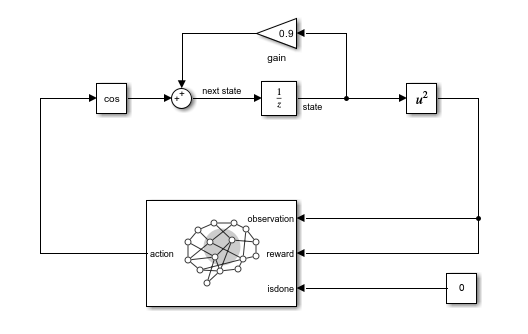
Implement the discrete-time system defined in dsStepFcn directly in Simulink. As discussed for the previous model, the delayed NextObs signal (that you connected to the agent observation input port in first Simulink model of this example), corresponds to the delayed square of the next state signal in the following model. This signal is identical (from the agent perspective) to the square of the current state signal.

Load the Simulink model in memory.

mdl = "dsLoopSDS";
load_system(mdl);

Define the agent block path within the model, and create the environment object.

blk = mdl + "/RL Agent";
slenv = rlSimulinkEnv(mdl,blk,oinfo,ainfo);

Simulate the environment, collecting the experience in the variable straj.

straj = sim(slenv,agentObj,simopts);

Display the action data.

straj.Action.act1.Data(:)'

ans = 1×6

    2.0636    1.3385    1.2263    1.1961    1.1869    1.1840

Display the observation data.

straj.Observation.obs1.Data(:)'

ans = 1×7

   25.0000   16.2159   14.8563   14.4907   14.3790   14.3437   14.3323

As expected, the trajectory is identical to the previous ones.

Implement the Same Environment in Continuous-Time

In this case, you can also replace the inner linear discrete-time system with its continuous-time equivalent, thereby relying on the Simulink solver to perform the integration step. This is shown in the next model. Note that in this case you do not have access to the next state and next observation signal.

Load and open the Simulink model with the continuous integrator.

mdl = "csLoop";
load_system(mdl);

Create the environment object

blk = mdl + "/RL Agent";
slenv = rlSimulinkEnv(mdl,blk,oinfo,ainfo);

Note that the Fixed-step ode1 (Euler) solver is selected in the Solver pane of the model configuration parameters.

Simulate the environment, collecting the experience in the variable straj.

straj = sim(slenv,agentObj,simopts);

Display the action data.

straj.Action.act1.Data(:)'

ans = 1×6

    2.0636    1.3385    1.2263    1.1961    1.1869    1.1840

Display the observation data.

straj.Observation.obs1.Data(:)'

ans = 1×7

   25.0000   16.2159   14.8563   14.4907   14.3790   14.3437   14.3323

Again, the trajectory is identical to the previous ones.

This example shows that when implementing an environment in Simulink, you have two options:

The second option is completely equivalent to the first one, but often simpler to use in cases in which the next state is not accessible, as for example for continuous-time environments.