Model RF Impairments in 5G NR Downlink Waveform

Since R2024b

This example uses:

This example shows how to model RF impairments introduced by a superheterodyne transmitter, such as phase noise, in-phase and quadrature (I/Q) imbalance, filter effects, and memoryless nonlinearity, on a 5G NR downlink waveform. It also shows how to measure the corresponding error vector magnitude (EVM).

Introduction

The example comprises these steps:

Generate a 5G NR downlink waveform defined by the 3GPP NR standard.
Model RF impairments as components of a superheterodyne transmitter.
Calculate the EVM of the 5G NR downlink waveform that is applied to the superheterodyne transmitter.

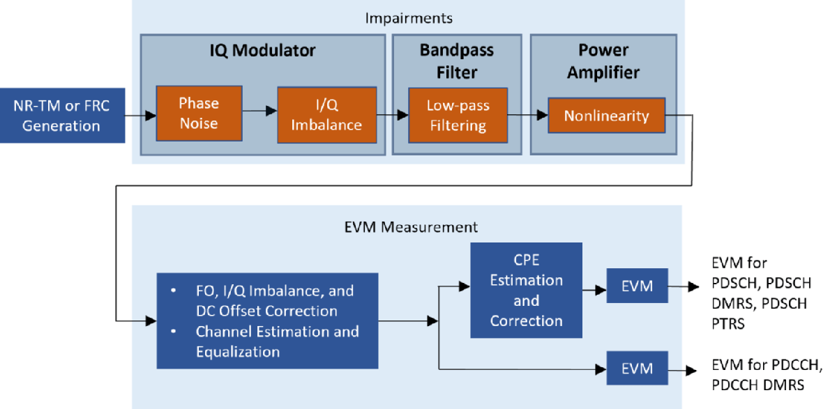
This figure shows the processing chain implemented in this example. For a more detailed discussion of the EVM measurement workflow, see the EVM Measurement of 5G NR Downlink Waveforms with RF Impairments (5G Toolbox) example.

Simulation Parameters

Simulation Parameters for 5G NR Downlink Waveform Generation

For RF testing of base stations, the 3GPP 5G NR standard specifies a series of NR test model (NR-TM) waveforms. For testing user equipment (UE), the standard outlines a set of fixed reference channel (FRC) waveforms. The NR-TMs and FRCs for frequency range 1 (FR1) are detailed in TS 38.141-1, whereas those for frequency range 2 (FR2) are described in TS 38.141-2.

Each FRC or NR-TM waveform is defined by a combination of these parameters:

NR-TM/FRC name
Channel bandwidth
Subcarrier spacing
Duplexing mode

Define simulation parameters for an NR downlink waveform defined by the 3GPP 5G NR standard.

rc = "NR-FR1-TM3.2"; % Reference channel (NR-TM or FRC)
% Select the NR waveform parameters
bw = "10MHz"; % Channel bandwidth
scs = "30kHz"; % Subcarrier spacing
dm = "FDD"; % Duplexing mode

For TMs, the generated waveform can contain more than one physical downlink shared channel (PDSCH). The chosen PDSCH to be analyzed is determined by the radio network temporary identifier (RNTI). By default, this example considers these RNTIs for EVM calculation with respect to the following TMs:

NR-FR1-TM2: RNTI = 2 (64QAM EVM)
NR-FR1-TM2a: RNTI = 2 (256QAM EVM)
NR-FR1-TM2b: RNTI = 2 (1024QAM EVM)
NR-FR1-TM3.1: RNTI = 0 and 2 (64QAM EVM)
NR-FR1-TM3.1a: RNTI = 0 and 2 (256QAM EVM)
NR-FR1-TM3.1b: RNTI = 0 and 2 (1024QAM EVM)
NR-FR1-TM3.2: RNTI = 1 (16QAM EVM)
NR-FR1-TM3.3: RNTI = 1 (QPSK EVM)
NR-FR2-TM2: RNTI = 2 (64QAM EVM)
NR-FR2-TM2a: RNTI = 2 (256QAM EVM)
NR-FR2-TM3.1: RNTI = 0 and 2 (64QAM EVM)
NR-FR2-TM3.1a: RNTI = 0 and 2 (256QAM EVM)

As per the specifications (TS 38.141-1, TS 38.141-2), these TMs are not designed to perform EVM measurements for conformance tests: NR-FR1-TM1.1, NR-FR1-TM1.2, NR-FR2-TM1.1. However, TMs are easy to generate and parameterize, so you can use them outside the scope of the test for which they were designed for, using their EVM measurements as a general methodology for assessing signal quality. If you generate these TMs, the algorithm used in the example measures the EVM for the following RNTIs:

NR-FR1-TM1.1: RNTI = 0 (QPSK EVM)
NR-FR1-TM1.2: RNTI = 2 (QPSK EVM)
NR-FR2-TM1.1: RNTI = 0 (QPSK EVM)

For PDSCH FRCs and physical downlink control channel (PDCCH), by default, RNTI 0 is considered for EVM calculation.

Calculate the PDSCH EVM for the RNTIs. To override the default PDSCH RNTIs, specify the targetRNTIs vector.

targetRNTIs = [];

Simulation Parameters for EVM Measurement

To print EVM statistics, select displayEVM.

displayEVM = true;

To plot EVM statistics, clear plotEVM.

plotEVM = true;

To measure EVM as defined in TS 38.104, Annex B(FR1) / Annex C(FR2), select evm3GPP.

evm3GPP = true;

Simulation Parameters for RF Impairments Modeling

This example considers the most common impairments that distort the waveform when it passes through an RF transmitter or receiver: phase noise, I/Q imbalance, filter effects, and memoryless nonlinearity. To enable or disable impairments, toggle the phaseNoiseOn, IQImbalanceOn, and nonLinearityModelOn flags. Define the distortion parameter values.

%#ok<*UNRCH>
% Set phase noise
phaseNoiseOn = true;
minFrequencyOffset = 1e4;

% Set I/Q imbalance
IQImbalanceOn = true;
amplitudeImbalance = 0.2;
phaseImbalance = 0.5;

% Set filtering
filterOn = true;

% Set amplifier gain
gain = 25; % Always on

% Set nonlinearity
nonLinearityModelOn = true;
rappMagnitudeSmooth = 1.15;
rappPhaseSaturation = 0.88;
rappPhaseSmooth = 3.43;

Furthermore, specify the modeling of white noise.

nfOn = true;
nf = 7;

Generate 5G NR Downlink Waveform

Before generating the 5G NR downlink waveform, specify a higher waveform sample rate to model wideband filter effects. You can increase the sample rate by multiplying the nominal sample rate with the oversampling factor, OSR. To use the nominal sample rate, set OSR to 1.

OSR = 5; % oversampling factor

% Create waveform generator object 
tmwavegen = hNRReferenceWaveformGenerator(rc,bw,scs,dm);

% Waveform bandwidth
bandwidth = tmwavegen.Config.ChannelBandwidth*1e6;

if OSR > 1
    % The |Config| property in |tmwavegen| specifies the configuration of
    % the standard-defined reference waveform. It is a read-only property.
    % To customize the waveform, make the |Config| property writable.
    tmwavegen = makeConfigWritable(tmwavegen);

    % Increase the waveform sample rate by multiplying the nominal sample
    % rate with |OSR|
    nominalSampleRate = getNominalSampleRate(tmwavegen.Config);
    tmwavegen.Config.SampleRate = nominalSampleRate*OSR;
else
    filterOn = false;
end

Now, generate the waveform and get the waveform sample rate.

[txWaveform,tmwaveinfo,resourcesinfo] = generateWaveform(tmwavegen,tmwavegen.Config.NumSubframes);
sr = tmwaveinfo.Info.SamplingRate; % waveform sample rate

Normalize the waveform to fit the dynamic range of the nonlinearity.

gain = 25;
peakPower = 10^(-gain/20);
txWaveform = peakPower.*txWaveform/max(abs(txWaveform),[],'all');

The waveform consists of one frame for frequency division duplex (FDD) and two for time division duplex (TDD). Repeat the signal twice. Remove the first half of the resulting waveform to avoid the transient introduced by the phase noise model.

txWaveform = repmat(txWaveform,2,1);

Transmitter with RF Impairments

This section shows how to model RF impairments as components of a superheterodyne transmitter. Using RF Toolbox™ Idealized Baseband library elements, add phase noise, I/Q imbalance, filter effects, and memoryless nonlinearity to model the effects of upconverting the waveform to the carrier frequency. There are two ways to model RF impairments: components-based and isolated impairments modeling. This example models impairments using component-based impairments modeling as shown in this figure. For more information on how to model the impairments as isolated constituents, see the EVM Measurement of 5G NR Downlink Waveforms with RF Impairments (5G Toolbox) example.

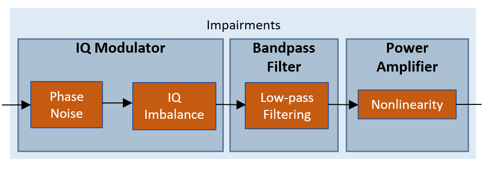
Build the superheterodyne transmitter architecture by characterizing these RF components:

IQ modulator
Bandpass filter (BPF)
Power amplifier

% Define frequency values
switch tmwavegen.Config.FrequencyRange
    case "FR1" % carrier frequency for FR1
        fc = 4e9;
    case "FR2" % carrier frequency for FR2
        fc = 30e9;
end

% Build transmitter
RFmixer = rf.Mixer('Model','iqmod');
RFfilter = rf.Filter('ResponseType','Bandpass', ...
    'UseFilterOrder',false, ...
    'PassFreq_bp',fc+[-(sr/2-(sr/2*0.6)) sr/2-(sr/2*0.6)], ...
    'PassAtten',0.7,...
    'StopFreq_bp',fc+[-(sr/2-(sr/2*0.5)) sr/2-(sr/2*0.5)], ...
    'StopAtten',60, ...
    'SampleRate',sr, ...
    'RF',fc);
RFHPA = rf.Amplifier('Gain',gain);

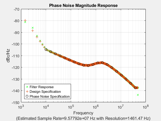
Add phase noise distortion. The phase noise characteristic is generated with the multipole zero model described in TR 38.803 Section 6.1.10. The figure shows the phase noise characteristic.

if phaseNoiseOn
    [level,frequencyOffset] = getPhaseNoisePSD(fc,sr,minFrequencyOffset);

    RFmixer.IncludePhaseNoise = true;
    RFmixer.PhaseNoiseLevel = level;
    RFmixer.PhaseNoiseFrequencyOffset = frequencyOffset;
    RFMixer.NoiseSeedSource = 'user';
    RFMixer.NoiseSeed = 2137;

    visualizePhaseNoise(RFmixer)
end

Figure RFmixer contains an axes object. The axes object with title Phase Noise Magnitude Response, xlabel Frequency (Estimated Sample Rate=9.57792e+07 Hz with Resolution=1461.47 Hz), ylabel dBc/Hz contains 3 objects of type line. One or more of the lines displays its values using only markers These objects represent Filter Response, Design Specification, Phase Noise Specification.

Add I/Q imbalance by applying a 0.2 dB amplitude imbalance and a 0.5 degree phase imbalance to the mixer. You can also increase the amplitude and phase imbalances by setting GainImbalance and PhaseImbalance to higher values.

if IQImbalanceOn
    RFMixer.GainImbalance = amplitudeImbalance;
    RFMixer.PhaseImbalance = phaseImbalance;
end

Filter the waveform by using a BPF and plot its magnitude response.

If the current passband and stopband frequencies result in high EVM values for a different waveform bandwidth and OSR, use a wider filter by increasing the parameters PassFreq_bp and StopFreq_bp in the Idealized Baseband filter block. To use a narrower filter, reduce PassFreq_bp and StopFreq_bp. You can also modify the passband ripple and the stopband attenuation. This figure shows the magnitude response of the BPF.

if filterOn
    RFfilter.FrequencyPoints = linspace(fc-sr,fc+sr,2001);

    visualize(RFfilter)
end

Figure contains an axes object. The axes object with xlabel Frequency [Hz], ylabel S21 [Mag (dB)] contains an object of type line.

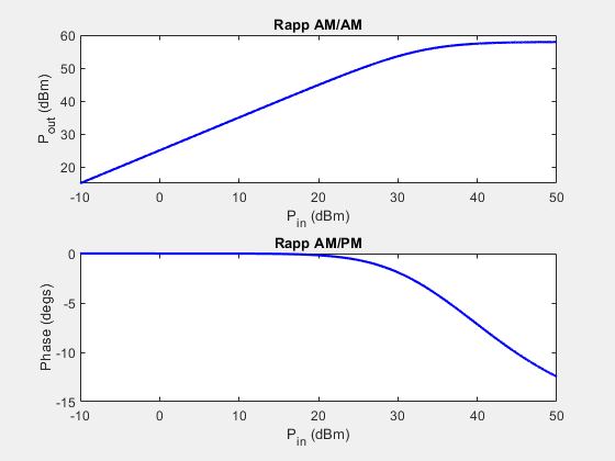
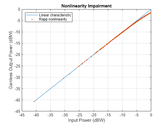
Introduce nonlinear distortion using the Rapp model in the power amplifier. Set the parameters for the Rapp model to match the characteristics of the memoryless model from TR 38.803 Annex A.1. These figures show the nonlinearity introduced by the Rapp model.

if nonLinearityModelOn
    RFHPA.Model = 'modified-rapp';

    RFHPA.MagnitudeGainDB = gain;
    RFHPA.Vsat = gain;
    RFHPA.MagnitudeSmooth = rappMagnitudeSmooth;

    RFHPA.PhaseSaturation = rappPhaseSaturation;
    RFHPA.PhaseSmooth = rappPhaseSmooth;

    visualize(RFHPA)
    plotNonLinearCharacteristic(RFHPA)
end

Figure RFHPA contains 2 axes objects. Axes object 1 with title Rapp AM/AM, xlabel P_i_n (dBm), ylabel P_o_u_t (dBm) contains an object of type line. Axes object 2 with title Rapp AM/PM, xlabel P_i_n (dBm), ylabel Phase (degs) contains an object of type line.

Figure contains an axes object. The axes object with title Nonlinearity Impairment, xlabel Input Power (dBW), ylabel Gainless Output Power (dBW) contains 2 objects of type line. One or more of the lines displays its values using only markers These objects represent Linear characteristic, Rapp nonlinearity.

Finally, introduce white noise in elements of the transmitter.

if nfOn
    % Speciy NF in IQ modulator
    RFmixer.IncludeNoise = true;
    RFmixer.NF = nf;

    % Specify NF in HPA
    RFHPA.IncludeNoise = true;
    RFHPA.NF = nf;
end

Simulate the impairments of the transmitter on the waveform.

out_iq = RFmixer(txWaveform);
release(RFmixer)

if filterOn
    out_filt = RFfilter(out_iq);
    release(RFfilter)
else
    out_filt = out_iq;
end

rxWaveform = RFHPA(out_filt);
release(RFHPA)

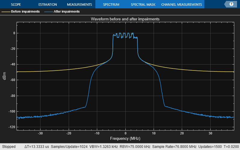
Plot the spectrum of the waveform before and after adding the RF impairments.

scope = spectrumAnalyzer('SampleRate',sr,...
    'ChannelNames',{'Before impairments','After impairments'},...
    'Title', 'Waveform before and after impairments');
scope([(1/peakPower).*txWaveform,rxWaveform]);
release(scope);

The signal was previously repeated twice. Remove the first half of this signal. This avoids any transient introduced by the impairment models.

nFrames = 1; % because dm = "FDD"
rxWaveform(1:nFrames*tmwaveinfo.Info.SamplesPerSubframe*10,:) = [];

Measure the EVM of the 5G NR Downlink Waveform

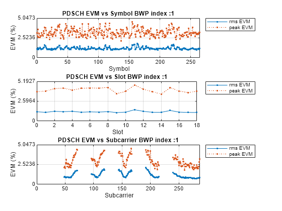
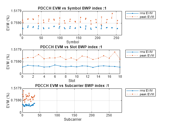
Calculate the EVM of the resulting signal. In this example, you plot the RMS and peak EVMs per orthogonal frequency division multiplexing (OFDM) symbol, slot, and subcarrier and calculate the overall EVM (RMS EVM averaged over the complete waveform). Annex B and Annex C of TS 38.104 define alternative methods for computing the EVM in FR1 and FR2, respectively. For detailed steps on the decoding and analysis of the waveform, see the description of the helper function hNRDownlinkEVM in the EVM Measurement of 5G NR Downlink Waveforms with RF Impairments (5G Toolbox) example.

cfg = struct();
cfg.Evm3GPP = evm3GPP;
cfg.TargetRNTIs = targetRNTIs;
cfg.PlotEVM = plotEVM;
cfg.DisplayEVM = displayEVM;
cfg.IQImbalance = IQImbalanceOn;

% Compute and display EVM measurements
[evmInfo,eqSym,refSym] = hNRDownlinkEVM(tmwavegen.Config,rxWaveform,cfg);

EVM stats for BWP idx : 1
Low edge PDSCH RMS EVM, Peak EVM, slot 0: 1.148 3.660%
Low edge DM-RS RMS EVM, Peak EVM, slot 0: 1.116 2.397%
High edge PDSCH RMS EVM, Peak EVM, slot 0: 1.142 3.884%
High edge DM-RS RMS EVM, Peak EVM, slot 0: 1.116 2.397%
Low edge PDSCH RMS EVM, Peak EVM, slot 1: 1.185 3.582%
Low edge DM-RS RMS EVM, Peak EVM, slot 1: 1.165 3.460%
High edge PDSCH RMS EVM, Peak EVM, slot 1: 1.187 3.564%
High edge DM-RS RMS EVM, Peak EVM, slot 1: 1.165 3.460%
Low edge PDSCH RMS EVM, Peak EVM, slot 2: 1.191 3.564%
Low edge DM-RS RMS EVM, Peak EVM, slot 2: 1.108 2.561%
High edge PDSCH RMS EVM, Peak EVM, slot 2: 1.190 3.543%
High edge DM-RS RMS EVM, Peak EVM, slot 2: 1.108 2.561%
Low edge PDSCH RMS EVM, Peak EVM, slot 3: 1.178 3.894%
Low edge DM-RS RMS EVM, Peak EVM, slot 3: 1.133 2.703%
High edge PDSCH RMS EVM, Peak EVM, slot 3: 1.175 4.074%
High edge DM-RS RMS EVM, Peak EVM, slot 3: 1.133 2.703%
Low edge PDSCH RMS EVM, Peak EVM, slot 4: 1.340 4.562%
Low edge DM-RS RMS EVM, Peak EVM, slot 4: 1.350 3.186%
High edge PDSCH RMS EVM, Peak EVM, slot 4: 1.341 4.555%
High edge DM-RS RMS EVM, Peak EVM, slot 4: 1.350 3.186%
Low edge PDSCH RMS EVM, Peak EVM, slot 5: 1.172 3.926%
Low edge DM-RS RMS EVM, Peak EVM, slot 5: 1.222 3.383%
High edge PDSCH RMS EVM, Peak EVM, slot 5: 1.165 3.775%
High edge DM-RS RMS EVM, Peak EVM, slot 5: 1.222 3.383%
Low edge PDSCH RMS EVM, Peak EVM, slot 6: 1.172 4.465%
Low edge DM-RS RMS EVM, Peak EVM, slot 6: 1.211 2.662%
High edge PDSCH RMS EVM, Peak EVM, slot 6: 1.172 4.360%
High edge DM-RS RMS EVM, Peak EVM, slot 6: 1.211 2.662%
Low edge PDSCH RMS EVM, Peak EVM, slot 7: 1.307 4.176%
Low edge DM-RS RMS EVM, Peak EVM, slot 7: 1.334 3.922%
High edge PDSCH RMS EVM, Peak EVM, slot 7: 1.314 4.209%
High edge DM-RS RMS EVM, Peak EVM, slot 7: 1.334 3.922%
Low edge PDSCH RMS EVM, Peak EVM, slot 8: 1.500 4.724%
Low edge DM-RS RMS EVM, Peak EVM, slot 8: 1.752 4.108%
High edge PDSCH RMS EVM, Peak EVM, slot 8: 1.498 4.833%
High edge DM-RS RMS EVM, Peak EVM, slot 8: 1.752 4.108%
Low edge PDSCH RMS EVM, Peak EVM, slot 9: 1.322 4.734%
Low edge DM-RS RMS EVM, Peak EVM, slot 9: 1.120 3.457%
High edge PDSCH RMS EVM, Peak EVM, slot 9: 1.325 4.770%
High edge DM-RS RMS EVM, Peak EVM, slot 9: 1.120 3.457%
Low edge PDSCH RMS EVM, Peak EVM, slot 10: 1.127 3.530%
Low edge DM-RS RMS EVM, Peak EVM, slot 10: 1.174 2.594%
High edge PDSCH RMS EVM, Peak EVM, slot 10: 1.136 3.589%
High edge DM-RS RMS EVM, Peak EVM, slot 10: 1.174 2.594%
Low edge PDSCH RMS EVM, Peak EVM, slot 11: 1.129 4.586%
Low edge DM-RS RMS EVM, Peak EVM, slot 11: 1.124 2.530%
High edge PDSCH RMS EVM, Peak EVM, slot 11: 1.129 4.582%
High edge DM-RS RMS EVM, Peak EVM, slot 11: 1.124 2.530%
Low edge PDSCH RMS EVM, Peak EVM, slot 12: 1.259 3.926%
Low edge DM-RS RMS EVM, Peak EVM, slot 12: 1.204 2.819%
High edge PDSCH RMS EVM, Peak EVM, slot 12: 1.261 4.065%
High edge DM-RS RMS EVM, Peak EVM, slot 12: 1.204 2.819%
Low edge PDSCH RMS EVM, Peak EVM, slot 13: 1.170 3.789%
Low edge DM-RS RMS EVM, Peak EVM, slot 13: 1.045 2.688%
High edge PDSCH RMS EVM, Peak EVM, slot 13: 1.170 3.744%
High edge DM-RS RMS EVM, Peak EVM, slot 13: 1.045 2.688%
Low edge PDSCH RMS EVM, Peak EVM, slot 14: 1.300 5.212%
Low edge DM-RS RMS EVM, Peak EVM, slot 14: 1.109 2.656%
High edge PDSCH RMS EVM, Peak EVM, slot 14: 1.297 5.096%
High edge DM-RS RMS EVM, Peak EVM, slot 14: 1.109 2.656%
Low edge PDSCH RMS EVM, Peak EVM, slot 15: 1.290 4.734%
Low edge DM-RS RMS EVM, Peak EVM, slot 15: 1.110 2.607%
High edge PDSCH RMS EVM, Peak EVM, slot 15: 1.289 4.690%
High edge DM-RS RMS EVM, Peak EVM, slot 15: 1.110 2.607%
Low edge PDSCH RMS EVM, Peak EVM, slot 16: 1.426 4.466%
Low edge DM-RS RMS EVM, Peak EVM, slot 16: 1.454 3.346%
High edge PDSCH RMS EVM, Peak EVM, slot 16: 1.428 4.434%
High edge DM-RS RMS EVM, Peak EVM, slot 16: 1.454 3.346%
Low edge PDSCH RMS EVM, Peak EVM, slot 17: 1.204 3.967%
Low edge DM-RS RMS EVM, Peak EVM, slot 17: 1.019 2.291%
High edge PDSCH RMS EVM, Peak EVM, slot 17: 1.206 3.999%
High edge DM-RS RMS EVM, Peak EVM, slot 17: 1.019 2.291%
Low edge PDSCH RMS EVM, Peak EVM, slot 18: 1.092 3.621%
Low edge DM-RS RMS EVM, Peak EVM, slot 18: 1.137 3.420%
High edge PDSCH RMS EVM, Peak EVM, slot 18: 1.095 3.640%
High edge DM-RS RMS EVM, Peak EVM, slot 18: 1.137 3.420%
PDCCH RMS EVM, Peak EVM, slot 0: 0.417 0.856%
PDCCH DM-RS RMS EVM, Peak EVM, slot 0: 0.257 0.475%
PDCCH RMS EVM, Peak EVM, slot 1: 0.555 1.203%
PDCCH DM-RS RMS EVM, Peak EVM, slot 1: 0.219 0.312%
PDCCH RMS EVM, Peak EVM, slot 2: 0.555 1.138%
PDCCH DM-RS RMS EVM, Peak EVM, slot 2: 0.267 0.540%
PDCCH RMS EVM, Peak EVM, slot 3: 0.538 1.344%
PDCCH DM-RS RMS EVM, Peak EVM, slot 3: 0.300 0.555%
PDCCH RMS EVM, Peak EVM, slot 4: 0.469 0.884%
PDCCH DM-RS RMS EVM, Peak EVM, slot 4: 0.270 0.417%
PDCCH RMS EVM, Peak EVM, slot 5: 0.494 1.246%
PDCCH DM-RS RMS EVM, Peak EVM, slot 5: 0.231 0.359%
PDCCH RMS EVM, Peak EVM, slot 6: 0.415 0.753%
PDCCH DM-RS RMS EVM, Peak EVM, slot 6: 0.231 0.394%
PDCCH RMS EVM, Peak EVM, slot 7: 0.527 1.243%
PDCCH DM-RS RMS EVM, Peak EVM, slot 7: 0.316 0.593%
PDCCH RMS EVM, Peak EVM, slot 8: 0.514 1.000%
PDCCH DM-RS RMS EVM, Peak EVM, slot 8: 0.221 0.431%
PDCCH RMS EVM, Peak EVM, slot 9: 0.552 1.615%
PDCCH DM-RS RMS EVM, Peak EVM, slot 9: 0.292 0.591%
PDCCH RMS EVM, Peak EVM, slot 10: 0.433 0.837%
PDCCH DM-RS RMS EVM, Peak EVM, slot 10: 0.233 0.373%
PDCCH RMS EVM, Peak EVM, slot 11: 0.481 1.106%
PDCCH DM-RS RMS EVM, Peak EVM, slot 11: 0.279 0.461%
PDCCH RMS EVM, Peak EVM, slot 12: 0.583 1.894%
PDCCH DM-RS RMS EVM, Peak EVM, slot 12: 0.294 0.484%
PDCCH RMS EVM, Peak EVM, slot 13: 0.442 0.864%
PDCCH DM-RS RMS EVM, Peak EVM, slot 13: 0.255 0.472%
PDCCH RMS EVM, Peak EVM, slot 14: 0.480 0.874%
PDCCH DM-RS RMS EVM, Peak EVM, slot 14: 0.203 0.362%
PDCCH RMS EVM, Peak EVM, slot 15: 0.538 1.443%
PDCCH DM-RS RMS EVM, Peak EVM, slot 15: 0.245 0.395%
PDCCH RMS EVM, Peak EVM, slot 16: 0.446 1.084%
PDCCH DM-RS RMS EVM, Peak EVM, slot 16: 0.188 0.302%
PDCCH RMS EVM, Peak EVM, slot 17: 0.501 0.939%
PDCCH DM-RS RMS EVM, Peak EVM, slot 17: 0.195 0.280%
PDCCH RMS EVM, Peak EVM, slot 18: 0.464 1.126%
PDCCH DM-RS RMS EVM, Peak EVM, slot 18: 0.276 0.406%

Figure EVM (%) contains an axes object. The axes object with title PDSCH EVM Resource Grid, BWP index : 1, xlabel OFDM symbols, ylabel Subcarriers contains an object of type surface.

Figure contains an axes object. The axes object with title PDSCH Equalized Symbols Constellation, BWP index : 1 contains 2 objects of type line. One or more of the lines displays its values using only markers

Figure EVM (%) contains an axes object. The axes object with title PDCCH EVM Resource Grid, BWP index : 1, xlabel OFDM symbols, ylabel Subcarriers contains an object of type surface.

Figure contains an axes object. The axes object with title PDCCH Equalized Symbols Constellation, BWP index : 1 contains 2 objects of type line. One or more of the lines displays its values using only markers

Averaged overall PDSCH RMS EVM: 1.242%
Overall PDSCH Peak EVM = 5.0955%
Averaged overall PDCCH RMS EVM: 0.497%
Overall PDCCH Peak EVM = 1.8939%

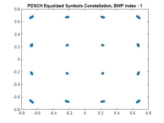
As per TS 38.104, the minimum requirement for the RMS EVM for QPSK/BPSK, 16QAM, 64QAM and 256QAM modulation must not exceed the EVM level of 17.5%, 12.5%, 8%, and 3.5%, respectively. This example's default waveform NR-FR1-TM3.2 utilizes 16QAM, and the printed EVM measurements indicate that the minimum requirement is met due to the PDSCH RMS EVM remaining below 12.5%.

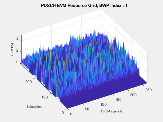
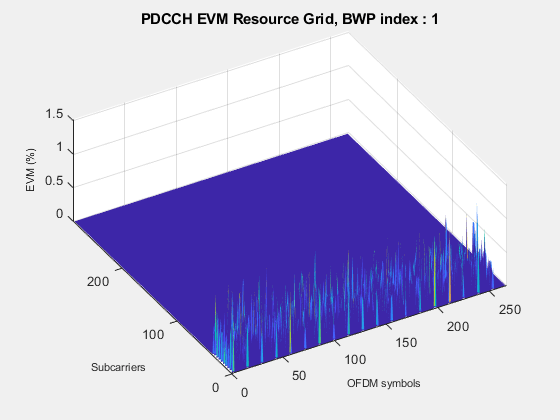
The EVM per OFDM symbol, per slot, per subcarrier, and resource grid plots help identify specific issues affecting the waveform's integrity:

The OFDM symbol plot can be analyzed to pinpoint precise moments when the signal integrity decreases to help identify adaptive modulation schemes that can apply real-time correction mechanisms.
The slot plot can give gain insight into broader fluctuations over time to address interference patterns or network conditions.
The subcarrier plot can be examined to identify frequency selective interference and fading to improve spectral efficiency.
The resource grid can be investigated to optimize scheduling algorithms and resource allocation strategies to minimize overall network errors.

In this example, the EVM across all plots must remain stable because the RF impairments modeled are temporally and spectrally independent.

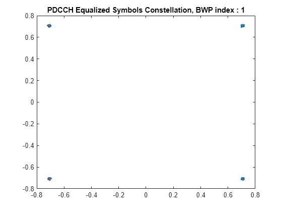
The constellation diagram helps diagnose random versus systematic issues. A widely dispersed contellation indicates high levels of noise or uncorrelated interference, whereas consistent deviations point to high non-linearity and I/Q imbalance.

References

[1] TR 38.803 V14.3.0. "Study on new radio access technology: Radio Frequency (RF) and co-existence aspects." 3rd Generation Partnership Project; Technical Specification Group Radio Access Network.

[2] TS 38.141-1. "NR; Base Station (BS) conformance testing Part 1: Conducted conformance testing." 3rd Generation Partnership Project; Technical Specification Group Radio Access Network.

[3] TS 38.141-2. "NR; Base Station (BS) conformance testing Part 2: Conducted conformance testing." 3rd Generation Partnership Project; Technical Specification Group Radio Access Network.

[4] TS 38.104. "NR; Base Station (BS) radio transmission and reception." 3rd Generation Partnership Project; Technical Specification Group Radio Access Network.

Local Functions

function [sampleRate] = getNominalSampleRate(cfgObj)
    % Obtain nominal sample rate for the input parameter CFGOBJ. CFGOBJ is
    % an object of type 'nrDLCarrierConfig'
    sampleRate = nr5g.internal.wavegen.maxSampleRate(cfgObj);
end

function [PN_dBcPerHz,fVec] = getPhaseNoisePSD(fc,sr,minFrequencyOffset)
    % Compute phase noise PSD for specified frequency offset fVec (in Hz) as
    % defined in TR 38.803
    
    fVec = logspace(log10(minFrequencyOffset),log10(sr/2)-0.001,20);
    [~,idx] = min(abs(fc - [29.55, 45, 70]*1e9));
    validMdl = {'29.55','45','70'};
    mdl = validMdl{idx};
    switch mdl
        case '29.55'
            % Parameter set from TR 38.803 for 29.55 GHz Fc
            fcBase = 29.55e9;
            fz = [3e3 550e3 280e6];
            fp = [1 1.6e6 30e6];
            alphaz = [2.37 2.7 2.53];
            alphap = [3.3 3.3 1];
            PSD0 = 32;
        case '45'
            % Parameter set from TR 38.803 for 45 GHz Fc
            fcBase = 45e9;
            fz = [3e3 451e3 458e6];
            fp = [1 1.54e6 30e6];
            alphaz = [2.37 2.7 2.53];
            alphap = [3.3 3.3 1];
            PSD0 = 35.65;
        otherwise
            % Parameter set from TR 38.803 for 70 GHz Fc
            fcBase = 70e9;
            fz = [3e3 396e3 754e6];
            fp = [1 1.55e6 30e6];
            alphaz = [2.37 2.7 2.53];
            alphap = [3.3 3.3 1];
            PSD0 = 39.49;
    end
    
    % Compute numerator
    num = ones(size(fVec));
    for ii = 1:numel(fz)
        num = num.*(1 + (fVec./fz(ii)).^alphaz(ii));
    end
    
    % Compute denominator
    den = ones(size(fVec));
    for ii = 1:numel(fp)
        den = den.*(1 + (fVec./fp(ii)).^alphap(ii));
    end
    
    % Compute phase noise and apply a shift for carrier frequencies
    % different from the base frequency
    PN_dBcPerHz = 10*log10(num./den) + PSD0 + 20*log10(fc/fcBase);
end

function plotNonLinearCharacteristic(RFHPA)
    % Plot the nonlinear characteristic of the power amplifier (PA) impairment.
    
    % Input samples
    x = complex((1/sqrt(2))*(-1+2*rand(1000,1)),(1/sqrt(2))*(-1+2*rand(1000,1)));

    % Nonlinearity
    yRapp = RFHPA(x);

    % Release object to feed it a different number of samples
    release(RFHPA);

    % Plot characteristic
    figure;
    plot(10*log10(abs(x).^2),10*log10(abs(x).^2));
    hold on;
    grid on
    plot(10*log10(abs(x).^2),10*log10(abs(yRapp).^2)-RFHPA.Gain,'.');
    xlabel('Input Power (dBW)');
    ylabel('Gainless Output Power (dBW)');
    title('Nonlinearity Impairment')
    legend('Linear characteristic', 'Rapp nonlinearity','Location','Northwest');
end