Expected Credit Loss Computation

Open Live Script

This example shows how to perform expected credit loss (ECL) computations with portfolioECL using simulated loan data, macro scenario data, and an existing lifetime probability of default (PD) model.

Load Data and Model

Load loan data ready for prediction, macro scenario data, and corresponding scenario probabilities.

load DataPredictLifetime.mat
disp(LoanData)

     ID      ScoreGroup      YOB    Year
    ____    _____________    ___    ____

    1304    "Medium Risk"     4     2020
    1304    "Medium Risk"     5     2021
    1304    "Medium Risk"     6     2022
    1304    "Medium Risk"     7     2023
    1304    "Medium Risk"     8     2024
    1304    "Medium Risk"     9     2025
    1304    "Medium Risk"    10     2026
    2067    "Low Risk"        7     2020
    2067    "Low Risk"        8     2021
    2067    "Low Risk"        9     2022
    2067    "Low Risk"       10     2023

disp(head(MultipleScenarios,10))

    ScenarioID    Year    GDP     Market
    __________    ____    ____    ______

    "Severe"      2020    -0.9     -5.5 
    "Severe"      2021    -0.5     -6.5 
    "Severe"      2022     0.2       -1 
    "Severe"      2023     0.8      1.5 
    "Severe"      2024     1.4        4 
    "Severe"      2025     1.8      6.5 
    "Severe"      2026     1.8      6.5 
    "Severe"      2027     1.8      6.5 
    "Adverse"     2020     0.1     -0.5 
    "Adverse"     2021     0.2     -2.5

disp(ScenarioProbabilities)

                 Probability
                 ___________

    Severe           0.1    
    Adverse          0.2    
    Baseline         0.3    
    Favorable        0.2    
    Excellent        0.2

load LifetimeChampionModel.mat
disp(pdModel)

  Probit with properties:

            ModelID: "Champion"
        Description: "A sample model used as champion model for illustration purposes."
    UnderlyingModel: [1x1 classreg.regr.CompactGeneralizedLinearModel]
              IDVar: "ID"
             AgeVar: "YOB"
           LoanVars: "ScoreGroup"
          MacroVars: ["GDP"    "Market"]
        ResponseVar: "Default"
         WeightsVar: ""
       TimeInterval: []

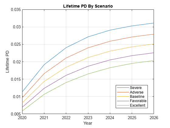
Visualize Lifetime PDs

For ECL computations, only the marginal PDs are required. However, first you can visualize the lifetime PDs.

CompanyIDChoice = "1304";
CompanyID = str2double(CompanyIDChoice);
IndCompany = LoanData.ID == CompanyID;
Years = LoanData.Year(IndCompany);
NumYears = length(Years);

ScenarioID = unique(MultipleScenarios.ScenarioID,'stable');
NumScenarios = length(ScenarioID);

LifetimePD = zeros(NumYears,NumScenarios);
for ii=1:NumScenarios
   IndScenario = MultipleScenarios.ScenarioID==ScenarioID(ii);
   data = join(LoanData(IndCompany,:),MultipleScenarios(IndScenario,:));
   LifetimePD(:,ii) = predictLifetime(pdModel,data);
end

plot(Years,LifetimePD)
xticks(Years)
grid on
xlabel('Year')
ylabel('Lifetime PD')
title('Lifetime PD By Scenario')
legend(ScenarioID,'Location','best')

Figure contains an axes object. The axes object with title Lifetime PD By Scenario, xlabel Year, ylabel Lifetime PD contains 5 objects of type line. These objects represent Severe, Adverse, Baseline, Favorable, Excellent.

Compute ECL

The computation of ECL requires a marginal PD values, LGD values, and EAD values, effective interest rate, plus the scenarios and scenario probabilities.

Compute the lifetime ECL using the portfolioECL function. The inputs to this function are tables, where the first column is an ID variable that indicates which rows correspond to which loan. Because the projections cover multiple periods for each loan, and the remaining life of different loans may be different, the ID variable is an important input. For each ID, the credit projections must be provided, period-by-period, until the end of the life of each loan. Typically, the marginal PD has a multi-period and multi-scenario size. This example assumes constant LGD and EAD values. This means that the same LGD and EAD is used for all periods, and the LGD and EAD values are not sensitive to the scenarios. Hence, the marginal PD input has multiple rows and columns per ID, whereas the LGD and EAD inputs have one scalar value per ID. To offer flexibility for different input dimensions for marginal PD, LGD, and EAD inputs, these inputs are separated into three separate tables in the syntax of portfolioECL.

ScenarioID = unique(MultipleScenarios.ScenarioID,'stable');
NumScenarios = length(ScenarioID);

Predict marginal PD for each scenario. The predictLifetime function is called for the entire portfolio at once, and the marginal PDs for each scenario are stored as columns.

MarginalPD = zeros(height(LoanData),NumScenarios);
for ii=1:NumScenarios
   IndScenario = MultipleScenarios.ScenarioID==ScenarioID(ii);
   data = join(LoanData,MultipleScenarios(IndScenario,:));
   MarginalPD(:,ii) = predictLifetime(pdModel,data,'ProbabilityType','marginal');
end

Convert to the required table input format, with the ID column.

MarginalPDTable = array2table(MarginalPD);
MarginalPDTable.Properties.VariableNames = ScenarioID;
MarginalPDTable = addvars(MarginalPDTable,LoanData.ID,'Before',1,'NewVariableNames','ID');
disp(MarginalPDTable)

     ID       Severe       Adverse       Baseline     Favorable     Excellent 
    ____    __________    __________    __________    __________    __________

    1304      0.011316     0.0096361     0.0081783      0.006918     0.0058324
    1304     0.0078277     0.0069482     0.0061554     0.0054425     0.0048028
    1304     0.0048869     0.0044693     0.0040823     0.0037243     0.0033938
    1304     0.0031017     0.0029321     0.0027698     0.0026147     0.0024668
    1304     0.0019309     0.0018923     0.0018538     0.0018153      0.001777
    1304     0.0012157     0.0012197     0.0012233     0.0012264     0.0012293
    1304    0.00082053    0.00082322    0.00082562    0.00082775    0.00082964
    2067     0.0022199      0.001832     0.0015067      0.001235     0.0010088
    2067     0.0014464     0.0012534     0.0010841    0.00093599    0.00080662
    2067     0.0008343    0.00074897    0.00067168    0.00060175    0.00053857
    2067    0.00049107    0.00045839    0.00042769    0.00039887    0.00037183

The LGD and EAD table inputs are small tables with one row per ID.

UniqueIDs = unique(LoanData.ID,'stable');
NumIDs = length(UniqueIDs);

LGD = 0.55;
LGDTable = table(UniqueIDs, repmat(LGD,NumIDs,1),'VariableNames',{'ID','LGD'});
disp(LGDTable)

     ID     LGD 
    ____    ____

    1304    0.55
    2067    0.55

EAD = 100000;
EADTable = table(UniqueIDs, repmat(EAD,NumIDs,1),'VariableNames',{'ID','EAD'});
disp(EADTable)

     ID      EAD 
    ____    _____

    1304    1e+05
    2067    1e+05

For simplicity, assume the same effective interest rate for both loans.

EffRate = 0.045;

Call the portfolioECL function. The first output is the total ECL, or provisions, for the portfolio.

[totalECL, ECLByID, ECLByPeriod] = portfolioECL(MarginalPDTable, LGDTable, EADTable, 'InterestRate', EffRate,...
    'ScenarioNames',ScenarioID, 'ScenarioProbabilities',ScenarioProbabilities.Probability, 'IDVar','ID','Periodicity','annual');

fprintf('Total portfolio lifetime ECL is: %.2f\n',totalECL)

Total portfolio lifetime ECL is: 1401.00

The second output, ECLByID, shows the ECL for each ID. The third output, ECLByPeriod, shows the ECL for each period, and each scenario. Use the dropdown to select an ID and display the corresponding ECL information.

CompanyIDChoice = "1304";
CompanyID = str2double(CompanyIDChoice);

disp(ECLByID(ECLByID.ID==CompanyID,:))

     ID      ECL  
    ____    ______

    1304    1217.3

disp(ECLByPeriod(ECLByPeriod.ID==CompanyID,:))

     ID     TimePeriod    Severe    Adverse    Baseline    Favorable    Excellent
    ____    __________    ______    _______    ________    _________    _________

    1304        1         595.58    507.16      430.44      364.11       306.97  
    1304        2         394.24    349.95      310.02      274.11        241.9  
    1304        3         235.53     215.4      196.75       179.5       163.57  
    1304        4         143.05    135.23      127.75      120.59       113.77  
    1304        5         85.219    83.517      81.816      80.118       78.429  
    1304        6         51.346    51.514      51.665      51.798       51.917  
    1304        7         33.162    33.271      33.368      33.454       33.531

For more information, see the Incorporate Macroeconomic Scenario Projections in Loan Portfolio ECL Calculations example that shows a detailed workflow for ECL calculations, including the determination of macro scenarios, the use of lifetime PD, LGD and EAD models, and a visualization of credit projections and provisions for each ID to drill down to a loan level.

Expected Credit Loss Computation

Load Data and Model

Visualize Lifetime PDs

Compute ECL

See Also

Related Topics