Main Content

modelCalibrationPlot

Plot observed default rates compared to predicted PDs on grouped data

Since R2023a

Description

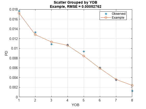
modelCalibrationPlot(pdModel,data,GroupBy) plots the observed default rates compared to the predicted probabilities of default (PD). GroupBy is required and can be any column in the data input (not necessarily a model variable). The modelCalibrationPlot function computes the observed PD as the default rate of each group and the predicted PD as the average PD for each group. modelCalibrationPlot supports comparison against a reference model.

example

modelCalibrationPlot(___,Name,Value) specifies options using one or more name-value pair arguments in addition to the input arguments in the previous syntax.

example

h = modelCalibrationPlot(ax,___,Name,Value) specifies options using one or more name-value pair arguments in addition to the input arguments in the previous syntax and returns the figure handle h.

example

Examples

collapse all

This example shows how to use modelCalibrationPlot to plot the root mean squared error (RMSE) of the observed probabilities of default (PDs) with respect to the predicted PDs.

Load Data

Load the credit portfolio data.

load RetailCreditPanelData.mat
disp(head(data))
    ID    ScoreGroup    YOB    Default    Year
    __    __________    ___    _______    ____

    1      Low Risk      1        0       1997
    1      Low Risk      2        0       1998
    1      Low Risk      3        0       1999
    1      Low Risk      4        0       2000
    1      Low Risk      5        0       2001
    1      Low Risk      6        0       2002
    1      Low Risk      7        0       2003
    1      Low Risk      8        0       2004
disp(head(dataMacro))
    Year     GDP     Market
    ____    _____    ______

    1997     2.72      7.61
    1998     3.57     26.24
    1999     2.86      18.1
    2000     2.43      3.19
    2001     1.26    -10.51
    2002    -0.59    -22.95
    2003     0.63      2.78
    2004     1.85      9.48

Join the two data components into a single data set.

data = join(data,dataMacro);
disp(head(data))
    ID    ScoreGroup    YOB    Default    Year     GDP     Market
    __    __________    ___    _______    ____    _____    ______

    1      Low Risk      1        0       1997     2.72      7.61
    1      Low Risk      2        0       1998     3.57     26.24
    1      Low Risk      3        0       1999     2.86      18.1
    1      Low Risk      4        0       2000     2.43      3.19
    1      Low Risk      5        0       2001     1.26    -10.51
    1      Low Risk      6        0       2002    -0.59    -22.95
    1      Low Risk      7        0       2003     0.63      2.78
    1      Low Risk      8        0       2004     1.85      9.48

Partition Data

Separate the data into training and test partitions.

nIDs = max(data.ID);
uniqueIDs = unique(data.ID);

rng('default'); % For reproducibility
c = cvpartition(nIDs,'HoldOut',0.4);

TrainIDInd = training(c);
TestIDInd = test(c);

TrainDataInd = ismember(data.ID,uniqueIDs(TrainIDInd));
TestDataInd = ismember(data.ID,uniqueIDs(TestIDInd));

Create Logistic Lifetime PD Model

Use fitLifetimePDModel to create a Logistic model using the training data.

pdModel = fitLifetimePDModel(data(TrainDataInd,:),'logistic',...
        'ModelID','Example',...
        'Description','Lifetime PD model using RetailCreditPanelData.',...
        'IDVar','ID',...
        'AgeVar','YOB',...
        'LoanVars','ScoreGroup',...
        'MacroVars',{'GDP' 'Market'},...
        'ResponseVar','Default');
 disp(pdModel)
  Logistic with properties:

            ModelID: "Example"
        Description: "Lifetime PD model using RetailCreditPanelData."
    UnderlyingModel: [1x1 classreg.regr.CompactGeneralizedLinearModel]
              IDVar: "ID"
             AgeVar: "YOB"
           LoanVars: "ScoreGroup"
          MacroVars: ["GDP"    "Market"]
        ResponseVar: "Default"
         WeightsVar: ""
       TimeInterval: 1
 pdModel.UnderlyingModel
ans = 
Compact generalized linear regression model:
    logit(Default) ~ 1 + ScoreGroup + YOB + GDP + Market
    Distribution = Binomial

Estimated Coefficients:
                               Estimate        SE         tStat       pValue   
                              __________    _________    _______    ___________

    (Intercept)                  -2.7422      0.10136    -27.054     3.408e-161
    ScoreGroup_Medium Risk      -0.68968     0.037286    -18.497     2.1894e-76
    ScoreGroup_Low Risk          -1.2587     0.045451    -27.693    8.4736e-169
    YOB                         -0.30894     0.013587    -22.738    1.8738e-114
    GDP                         -0.11111     0.039673    -2.8006      0.0051008
    Market                    -0.0083659    0.0028358    -2.9502      0.0031761


388097 observations, 388091 error degrees of freedom
Dispersion: 1
Chi^2-statistic vs. constant model: 1.85e+03, p-value = 0

Visualize Model Calibration

Use modelCalibrationPlot to visualize the model calibration on test data, grouping by age.

modelCalibrationPlot(pdModel,data(TestDataInd,:),'YOB')

Figure contains an axes object. The axes object with title Scatter Grouped by YOB Example, RMSE = 0.00052762, xlabel YOB, ylabel PD contains 2 objects of type line. One or more of the lines displays its values using only markers These objects represent Observed, Example.

Input Arguments

collapse all

Probability of default model, specified as a Logistic, Probit, or Cox object previously created using fitLifetimePDModel. Alternatively, you can create a custom probability of default model using customLifetimePDModel.

Note

The 'ModelID' property of the pdModel object is used as the identifier or tag for pdModel.

Data Types: object

Data, specified as a NumRows-by-NumCols table with projected predictor values to make lifetime predictions. The predictor names and data types must be consistent with the underlying model.

Data Types: table

Name of column in the data input used to group the data, specified as a string or character vector. GroupBy does not have to be a model variable name. For each group designated by GroupBy, the modelCalibrationPlot function computes the observed default rates and average predicted PDs are computed to measure the RMSE. modelCalibrationPlot supports up to two grouping variables.

Data Types: string | char

(Optional) Valid axis object, specified as an ax object that is created using axes. The plot will be created in the axes specified by the optional ax argument instead of in the current axes (gca). The optional argument ax must precede any of the input argument combinations.

Data Types: object

Name-Value Arguments

Specify optional pairs of arguments as Name1=Value1,...,NameN=ValueN, where Name is the argument name and Value is the corresponding value. Name-value arguments must appear after other arguments, but the order of the pairs does not matter.

Example: modelCalibrationPlot(pdModel,data(Ind,:),GroupBy=["YOB","ScoreGroup"],DataID="DataSetChoice")

Data set identifier, specified as DataID and a character vector or string. DataID is included in the plot title for reporting purposes.

Data Types: char | string

Conditional PD values predicted for data by the reference model, specified as ReferencePD and a NumRows-by-1 numeric vector. The predicted PD is plotted for both the pdModel object and the reference model.

Data Types: double

Identifier for the reference model, specified as ReferenceID and a character vector or string. ReferenceID is used in the plot for reporting purposes.

Data Types: char | string

Output Arguments

collapse all

Figure handle for the line objects, returned as handle object.

More About

collapse all

Model Calibration

Model calibration measures the accuracy of the predicted probability of default (PD) values.

The modelCalibrationPlot function allows you to visually compare the predicted PD values to the observed default rates. The modelCalibrationPlot function requires a grouping variable to compute average predicted PD values within each group and the average observed default rate also within each group. The predicted PD values and the observed default rates by group are plotted against the grouping variable values.

Up to two grouping variables are supported in modelCalibrationPlot. When two grouping variables are specified, the average predicted PD and default rates are computed for all the groups defined by the combination of the two grouping variables. The data is plotted against the first grouping variable, and the second variable is used to differentiate the data on the plot with different colors.

The root mean square error (RMSE) of the grouped data is reported on the title of the plot. To get the RMSE metric programmatically, use modelCalibration.

References

[1] Baesens, Bart, Daniel Roesch, and Harald Scheule. Credit Risk Analytics: Measurement Techniques, Applications, and Examples in SAS. Wiley, 2016.

[2] Bellini, Tiziano. IFRS 9 and CECL Credit Risk Modelling and Validation: A Practical Guide with Examples Worked in R and SAS. San Diego, CA: Elsevier, 2019.

[3] Breeden, Joseph. Living with CECL: The Modeling Dictionary. Santa Fe, NM: Prescient Models LLC, 2018.

[4] Roesch, Daniel and Harald Scheule. Deep Credit Risk: Machine Learning with Python. Independently published, 2020.

Version History

Introduced in R2023a