predict

Compute conditional PD

Since R2020b

collapse all in page

Syntax

conditionalPD = predict(pdModel,data)

Description

conditionalPD = predict(pdModel,data) computes the conditional probability of default (PD).

example

Examples

collapse all

Use Probit Lifetime PD Model to Predict Conditional PD

Open Live Script

This example shows how to use fitLifetimePDModel to fit data with a Probit model and then predict the conditional probability of default (PD).

Load Data

Load the credit portfolio data.

load RetailCreditPanelData.mat
disp(head(data))

    ID    ScoreGroup    YOB    Default    Year
    __    __________    ___    _______    ____

    1      Low Risk      1        0       1997
    1      Low Risk      2        0       1998
    1      Low Risk      3        0       1999
    1      Low Risk      4        0       2000
    1      Low Risk      5        0       2001
    1      Low Risk      6        0       2002
    1      Low Risk      7        0       2003
    1      Low Risk      8        0       2004

disp(head(dataMacro))

    Year     GDP     Market
    ____    _____    ______

    1997     2.72      7.61
    1998     3.57     26.24
    1999     2.86      18.1
    2000     2.43      3.19
    2001     1.26    -10.51
    2002    -0.59    -22.95
    2003     0.63      2.78
    2004     1.85      9.48

Join the two data components into a single data set.

data = join(data,dataMacro);
disp(head(data))

    ID    ScoreGroup    YOB    Default    Year     GDP     Market
    __    __________    ___    _______    ____    _____    ______

    1      Low Risk      1        0       1997     2.72      7.61
    1      Low Risk      2        0       1998     3.57     26.24
    1      Low Risk      3        0       1999     2.86      18.1
    1      Low Risk      4        0       2000     2.43      3.19
    1      Low Risk      5        0       2001     1.26    -10.51
    1      Low Risk      6        0       2002    -0.59    -22.95
    1      Low Risk      7        0       2003     0.63      2.78
    1      Low Risk      8        0       2004     1.85      9.48

Partition Data

Separate the data into training and test partitions.

nIDs = max(data.ID);
uniqueIDs = unique(data.ID);

rng('default'); % for reproducibility
c = cvpartition(nIDs,'HoldOut',0.4);

TrainIDInd = training(c);
TestIDInd = test(c);

TrainDataInd = ismember(data.ID,uniqueIDs(TrainIDInd));
TestDataInd = ismember(data.ID,uniqueIDs(TestIDInd));

Create a Probit Lifetime PD Model

Use fitLifetimePDModel to create a Probit model.

pdModel = fitLifetimePDModel(data(TrainDataInd,:),"Probit",...
    'AgeVar','YOB',...
    'IDVar','ID',...
    'LoanVars','ScoreGroup',...
    'MacroVars',{'GDP','Market'},...
    'ResponseVar','Default');
disp(pdModel)

  Probit with properties:

            ModelID: "Probit"
        Description: ""
    UnderlyingModel: [1x1 classreg.regr.CompactGeneralizedLinearModel]
              IDVar: "ID"
             AgeVar: "YOB"
           LoanVars: "ScoreGroup"
          MacroVars: ["GDP"    "Market"]
        ResponseVar: "Default"
         WeightsVar: ""
       TimeInterval: 1

Display the underlying model.

pdModel.UnderlyingModel

ans = 
Compact generalized linear regression model:
    probit(Default) ~ 1 + ScoreGroup + YOB + GDP + Market
    Distribution = Binomial

Estimated Coefficients:
                               Estimate        SE         tStat       pValue   
                              __________    _________    _______    ___________

    (Intercept)                  -1.6267      0.03811    -42.685              0
    ScoreGroup_Medium Risk      -0.26542      0.01419    -18.704     4.5503e-78
    ScoreGroup_Low Risk         -0.46794     0.016364    -28.595     7.775e-180
    YOB                         -0.11421    0.0049724    -22.969    9.6208e-117
    GDP                        -0.041537     0.014807    -2.8052      0.0050291
    Market                    -0.0029609    0.0010618    -2.7885      0.0052954


388097 observations, 388091 error degrees of freedom
Dispersion: 1
Chi^2-statistic vs. constant model: 1.85e+03, p-value = 0

Predict on Training and Test Data

Predict the PD for training or test data sets.

DataSetChoice = "Training";
if DataSetChoice=="Training"
    Ind = TrainDataInd;
 else
    Ind = TestDataInd;
 end

% Predict conditional PD
PD = predict(pdModel,data(Ind,:));
head(data(Ind,:))

    ID    ScoreGroup    YOB    Default    Year     GDP     Market
    __    __________    ___    _______    ____    _____    ______

    1      Low Risk      1        0       1997     2.72      7.61
    1      Low Risk      2        0       1998     3.57     26.24
    1      Low Risk      3        0       1999     2.86      18.1
    1      Low Risk      4        0       2000     2.43      3.19
    1      Low Risk      5        0       2001     1.26    -10.51
    1      Low Risk      6        0       2002    -0.59    -22.95
    1      Low Risk      7        0       2003     0.63      2.78
    1      Low Risk      8        0       2004     1.85      9.48

disp(PD(1:8))

You can analyze and validate these predictions using modelDiscrimination and modelCalibration.

Use Cox Lifetime PD Model to Predict Conditional PD

Open Live Script

This example shows how to use fitLifetimePDModel to fit data with a Cox model and then predict the conditional probability of default (PD).

Load Data

Load the credit portfolio data.

load RetailCreditPanelData.mat
disp(head(data))

    ID    ScoreGroup    YOB    Default    Year
    __    __________    ___    _______    ____

    1      Low Risk      1        0       1997
    1      Low Risk      2        0       1998
    1      Low Risk      3        0       1999
    1      Low Risk      4        0       2000
    1      Low Risk      5        0       2001
    1      Low Risk      6        0       2002
    1      Low Risk      7        0       2003
    1      Low Risk      8        0       2004

disp(head(dataMacro))

    Year     GDP     Market
    ____    _____    ______

    1997     2.72      7.61
    1998     3.57     26.24
    1999     2.86      18.1
    2000     2.43      3.19
    2001     1.26    -10.51
    2002    -0.59    -22.95
    2003     0.63      2.78
    2004     1.85      9.48

Join the two data components into a single data set.

data = join(data,dataMacro);
disp(head(data))

    ID    ScoreGroup    YOB    Default    Year     GDP     Market
    __    __________    ___    _______    ____    _____    ______

    1      Low Risk      1        0       1997     2.72      7.61
    1      Low Risk      2        0       1998     3.57     26.24
    1      Low Risk      3        0       1999     2.86      18.1
    1      Low Risk      4        0       2000     2.43      3.19
    1      Low Risk      5        0       2001     1.26    -10.51
    1      Low Risk      6        0       2002    -0.59    -22.95
    1      Low Risk      7        0       2003     0.63      2.78
    1      Low Risk      8        0       2004     1.85      9.48

Partition Data

Separate the data into training and test partitions.

nIDs = max(data.ID);
uniqueIDs = unique(data.ID);

rng('default'); % for reproducibility
c = cvpartition(nIDs,'HoldOut',0.4);

TrainIDInd = training(c);
TestIDInd = test(c);

TrainDataInd = ismember(data.ID,uniqueIDs(TrainIDInd));
TestDataInd = ismember(data.ID,uniqueIDs(TestIDInd));

Create a Cox Lifetime PD Model

Use fitLifetimePDModel to create a Cox model.

ModelType = "cox";

pdModel = fitLifetimePDModel(data(TrainDataInd,:),ModelType,...
   'IDVar','ID','AgeVar','YOB',...
   'LoanVars','ScoreGroup','MacroVars',{'GDP' 'Market'},...
   'ResponseVar','Default');
disp(pdModel)

  Cox with properties:

    ExtrapolationFactor: 1
                ModelID: "Cox"
            Description: ""
        UnderlyingModel: [1x1 CoxModel]
                  IDVar: "ID"
                 AgeVar: "YOB"
               LoanVars: "ScoreGroup"
              MacroVars: ["GDP"    "Market"]
            ResponseVar: "Default"
             WeightsVar: ""
           TimeInterval: 1

Display the underlying model.

disp(pdModel.UnderlyingModel)

Cox Proportional Hazards regression model

                                 Beta          SE         zStat       pValue   
                              __________    _________    _______    ___________

    ScoreGroup_Medium Risk       -0.6794     0.037029    -18.348     3.4442e-75
    ScoreGroup_Low Risk          -1.2442     0.045244    -27.501    1.7116e-166
    GDP                        -0.084533     0.043687     -1.935       0.052995
    Market                    -0.0084411    0.0032221    -2.6198      0.0087991


Log-likelihood: -41742.871

Predict on Age Values not Observed in the Training Data

Cox models make predictions for the range of age values observed in the training data. To extrapolate for ages larger than the maximum age in the training data, an extrapolation rule is needed.

When using predict with a Cox model, you can set the ExtrapolationFactor property of the Cox model. By default, the ExtrapolationFactor is set to 1. For age values (AgeVar) greater than the maximum age observed in the training data, predict computes the conditional PD using the maximum age observed in the training data. In particular, the predicted PD value is constant if the predictor values do not change and only the age values change when the ExtrapolationFactor is 1.

To illustrate this, select the rows corresponding to a single ID and add new rows with new, incremental age values beyond the maximum observed age in the training data. The maximum age observed in the training data is 8; for illustration purposes, add rows with ages 9, 10, 11, and 12.

% Select rows corresponding to one ID
% ID 1 goes from row 1 through 8
% Only the ID, Age (YOB) and predictor variables are needed
dataNewAge = data(1:8,{'ID' 'YOB' 'ScoreGroup' 'GDP' 'Market'});
% Allocate more rows
% This line copies the same predictor values going forward
dataNewAge(9:12,:) = repmat(dataNewAge(8,:),4,1);
% Reset age values to 9, 10, 11, 12
dataNewAge.YOB(9:12) = (9:12)';
% Show the new dataset
disp(dataNewAge)

    ID    YOB    ScoreGroup     GDP     Market
    __    ___    __________    _____    ______

    1      1      Low Risk      2.72      7.61
    1      2      Low Risk      3.57     26.24
    1      3      Low Risk      2.86      18.1
    1      4      Low Risk      2.43      3.19
    1      5      Low Risk      1.26    -10.51
    1      6      Low Risk     -0.59    -22.95
    1      7      Low Risk      0.63      2.78
    1      8      Low Risk      1.85      9.48
    1      9      Low Risk      1.85      9.48
    1     10      Low Risk      1.85      9.48
    1     11      Low Risk      1.85      9.48
    1     12      Low Risk      1.85      9.48

When the predictor values are constant in the rows with new age values and the extrapolation factor is 1, the predicted PD values are constant. If the extrapolation factor is set to a value smaller than 1, then the predicted PD values decrease more and more for larger age values and decrease towards zero exponentially.

% Extrapolation factor can be adjusted
pdModel.ExtrapolationFactor = 1;
% Store predicted conditional PD in the same table
dataNewAge.PD = predict(pdModel,dataNewAge);
disp(dataNewAge)

    ID    YOB    ScoreGroup     GDP     Market        PD    
    __    ___    __________    _____    ______    __________

    1      1      Low Risk      2.72      7.61     0.0092197
    1      2      Low Risk      3.57     26.24      0.005158
    1      3      Low Risk      2.86      18.1     0.0046079
    1      4      Low Risk      2.43      3.19     0.0041351
    1      5      Low Risk      1.26    -10.51      0.003645
    1      6      Low Risk     -0.59    -22.95     0.0041128
    1      7      Low Risk      0.63      2.78     0.0017034
    1      8      Low Risk      1.85      9.48    0.00092551
    1      9      Low Risk      1.85      9.48    0.00092551
    1     10      Low Risk      1.85      9.48    0.00092551
    1     11      Low Risk      1.85      9.48    0.00092551
    1     12      Low Risk      1.85      9.48    0.00092551

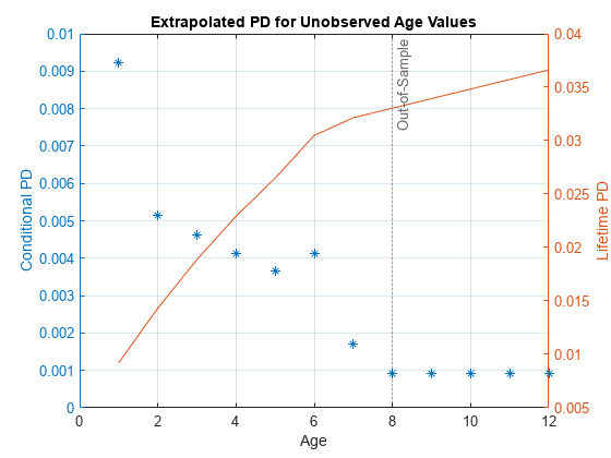
Also, it is useful to see the effect of the extrapolation factor on the lifetime prediction.

Plot the predicted conditional PD values and the lifetime PD values to see the effect of the extrapolation factor on both probabilities. The vertical dotted line separates the known age values (up to, and including, the age value 8), from the age values not observed in the training data (anything greater than 8). If the extrapolation factor is 1, the lifetime PD has a steady upward trend and the conditional PDs are constant. If the extrapolation factor is set to a smaller value like 0.5, the lifetime PD flattens quickly, as the conditional PD quickly drops towards zero.

dataNewAge.LifetimePD = predictLifetime(pdModel,dataNewAge);

figure;
yyaxis left
plot(dataNewAge.YOB,dataNewAge.PD,'*')
ylabel('Conditional PD')
yyaxis right
plot(dataNewAge.YOB,dataNewAge.LifetimePD)
ylabel('Lifetime PD')
title('Extrapolated PD for Unobserved Age Values')
xlabel('Age')
xline(8,':','Out-of-Sample')
grid on

Figure contains an axes object. The axes object with title Extrapolated PD for Unobserved Age Values, xlabel Age, ylabel Lifetime PD contains 3 objects of type line, constantline. One or more of the lines displays its values using only markers

Input Arguments

collapse all

`pdModel` — Probability of default model
`Logistic` object | `Probit` object | `Cox` object | `customLifetimePDModel` object

Probability of default model, specified as a previously created Logistic, Probit, or Cox object using fitLifetimePDModel. Alternatively, you can create a custom probability of default model using customLifetimePDModel.

Data Types: object

`data` — Data
table

Data, specified as a NumRows-by-NumCols table with projected predictor values to make lifetime predictions. The predictor names and data types must be consistent with the underlying model.

Data Types: table

Output Arguments

collapse all

`conditionalPD` — Predicted conditional probability of default values
vector

Predicted conditional probability of default values, returned as a NumRows-by-1 numeric vector.

More About

collapse all

Conditional PD

Conditional PD is the probability of defaulting, given no default yet.

For example, the predicted conditional PD for the second year is the probability that the borrower defaults in the second year, given that the borrower did not default in the first year.

The formula for conditional PD is

$P D (t) = P {t - Δ t < T \leq t | T > t - Δ t}$

where

T is the time to default.
Δt is the "time interval" consistent with the periodicity of the panel training data (for example, one row per year) and the definition of the default indicator values.

The default indicator is 1 if there is a default over a 1-year period. For more information on time intervals, see Time Interval for Logistic Models, Time Interval for Probit Models, and Time Interval for Cox Models.

In the formulas that follow for Logistic, Probit, and Cox models, the notation is:

X(t) is the predictor data for the row corresponding to time t.
β is the vector of coefficients of the underlying model.

For Logistic models, the conditional PD is computed as:

$P D_{c o n d} (t) = \frac{1}{1 + \exp (- X (t) β)}$

For Probit models, the conditional PD is computed as:

$P D_{c o n d} (t) = ϕ (X (t) β)$

For Cox models, the conditional PD is computed as

$P D_{c o n d} (t) = 1 - \frac{S (t)}{S (t - Δ t)}$

where S is the survival function. The survival function depends on the predictor values through the hazard ratio. For more information, see Cox Proportional Hazards Models. There are different ways to represent the dependence of the PD on the predictors explicitly. The implementation in the predict function uses the baseline cumulative hazard rate function given by

$H_{0} (t) = \int_{0}^{t} h_{0} (u) d u$

where h₀ is the baseline hazard rate. For more information, see Cox Proportional Hazards Models. Using the baseline cumulative hazard rate, the PD formula for the Cox model is written as:

$P D_{c o n d} (t) = 1 - \exp (- (H_{0} (t) - H_{0} (t - Δ t)) \exp (X (t) β))$

Extrapolation for `Cox` Models

The baseline cumulative hazard function H₀ for Cox models is fitted to the observed age values (that is, the observed "times-to-event") in a nonparametric way.

Therefore, some form of interpolation or extrapolation is needed to make predictions for age values not observed in the training data. In the predict function, linear interpolation is used as follows:

If the known age values are t₁, t₂,...,t_N, with t_i - t_{i -1} = Δt, and if t₀ = t₁ - Δt, then:
- H₀(t) = 0, for all t ≤ t₀.
- H₀(t) is interpolated linearly for t_{i
  -1} ≤ t ≤ t_i, for i = 0,...N.
- H₀(t) is extrapolated linearly for t > t_N, following the slope defined by the last two known values H₀(t_{N
  - 1}) and H₀(t_N).

This implies the baseline hazard rate h₀ is piecewise constant and remains constant after the last fitted value. By default, after the last known age value, the PD is evaluated as follows

$P D_{c o n d} (t | X (t)) = P D_{c o n d} (t_{N} | X (t))$

for t > t_N. This behavior is adjusted with the ExtrapolationFactor property of the Cox model. For more information, see Use Cox Lifetime PD Model to Predict Conditional PD.

Extrapolation Factor for `Cox` Models

The extrapolation formula implemented in the predict function includes the ExtrapolationFactor property value

$P D_{c o n d} (t_{N + k} | X (t_{N + k})) = {(E x t r a p o l a t i o n F a c t o r)}^{k} P D_{c o n d} (t_{N} | X (t_{N + k}))$

where t_{N +
k} is the time value k periods after the largest age observed in the training data t_N, that is, t_{N +
k} = t_N + k* Δt.

By default, the extrapolation factor is 1, resulting in the formula in the Extrapolation for Cox Models section, where the PD values remain constant as the age increases — if the predictor values do not change. If the extrapolation factor is set to a value smaller than 1, the predicted PD values decrease exponentially towards 0. The smaller the factor, the faster the conditional PD values decrease, and the faster the lifetime PD values flatten out.

In general, PD values tend to go down towards the end of the life of a loan, since the pool of borrowers gets cured earlier on. How fast this happens depends on the product and must be calibrated on a case-by-case basis.

Note that Logistic and Probit models need no special considerations regarding interpolation or extrapolation. These models are fully parametric models and predict the conditional PD for any values, in between, or beyond the numeric values observed in the dataset.

References

[1] Baesens, Bart, Daniel Roesch, and Harald Scheule. Credit Risk Analytics: Measurement Techniques, Applications, and Examples in SAS. Wiley, 2016.

[2] Bellini, Tiziano. IFRS 9 and CECL Credit Risk Modelling and Validation: A Practical Guide with Examples Worked in R and SAS. San Diego, CA: Elsevier, 2019.

[3] Breeden, Joseph. Living with CECL: The Modeling Dictionary. Santa Fe, NM: Prescient Models LLC, 2018.

[4] Roesch, Daniel and Harald Scheule. Deep Credit Risk: Machine Learning with Python. Independently published, 2020.

Version History

Introduced in R2020b

expand all

R2022b: Support for `customLifetimePDModel` model

The pdModel input supports an option for a customLifetimePDModel model object that you can create using customLifetimePDModel.

predict

Syntax

Description

Examples

Use Probit Lifetime PD Model to Predict Conditional PD

Use Cox Lifetime PD Model to Predict Conditional PD

Input Arguments

`pdModel` — Probability of default model
`Logistic` object | `Probit` object | `Cox` object | `customLifetimePDModel` object

`data` — Data
table

Output Arguments

`conditionalPD` — Predicted conditional probability of default values
vector

More About

Conditional PD

Extrapolation for `Cox` Models

Extrapolation Factor for `Cox` Models

References

Version History

R2022b: Support for `customLifetimePDModel` model

See Also

Topics

predict

Syntax

Description

Examples

Use Probit Lifetime PD Model to Predict Conditional PD

Use Cox Lifetime PD Model to Predict Conditional PD

Input Arguments

pdModel — Probability of default model Logistic object | Probit object | Cox object | customLifetimePDModel object

data — Data table

Output Arguments

conditionalPD — Predicted conditional probability of default values vector

More About

Conditional PD

Extrapolation for Cox Models

Extrapolation Factor for Cox Models

References

Version History

R2022b: Support for customLifetimePDModel model

See Also

Topics

`pdModel` — Probability of default model
`Logistic` object | `Probit` object | `Cox` object | `customLifetimePDModel` object

`data` — Data
table

`conditionalPD` — Predicted conditional probability of default values
vector

Extrapolation for `Cox` Models

Extrapolation Factor for `Cox` Models

R2022b: Support for `customLifetimePDModel` model