Compare Model Discrimination and Model Calibration to Validate of Probability of Default

Load and Fit Data

Load credit data and fit a Logistic lifetime PD model using fitLifetimePDModel.

load RetailCreditPanelData.mat
data = join(data,dataMacro);
pdModel = fitLifetimePDModel(data,"logistic",...
    'AgeVar','YOB',...
    'IDVar','ID',...
    'LoanVars','ScoreGroup',...
    'MacroVars',{'GDP','Market'},...
    'ResponseVar','Default');
disp(pdModel)

  Logistic with properties:

            ModelID: "Logistic"
        Description: ""
    UnderlyingModel: [1x1 classreg.regr.CompactGeneralizedLinearModel]
              IDVar: "ID"
             AgeVar: "YOB"
           LoanVars: "ScoreGroup"
          MacroVars: ["GDP"    "Market"]
        ResponseVar: "Default"
         WeightsVar: ""
       TimeInterval: 1

disp(pdModel.UnderlyingModel)

Compact generalized linear regression model:
    logit(Default) ~ 1 + ScoreGroup + YOB + GDP + Market
    Distribution = Binomial

Estimated Coefficients:
                               Estimate        SE         tStat       pValue   
                              __________    _________    _______    ___________

    (Intercept)                  -2.6799     0.078374    -34.193    3.0262e-256
    ScoreGroup_Medium Risk      -0.69409     0.028701    -24.184    3.2931e-129
    ScoreGroup_Low Risk          -1.2979     0.035548    -36.511    7.4134e-292
    YOB                         -0.31534     0.010529    -29.949    4.5479e-197
    GDP                           -0.128      0.03068    -4.1723     3.0157e-05
    Market                    -0.0073407    0.0021916    -3.3496     0.00080942


646724 observations, 646718 error degrees of freedom
Dispersion: 1
Chi^2-statistic vs. constant model: 3.2e+03, p-value = 0

Same Discrimination, Different Calibration

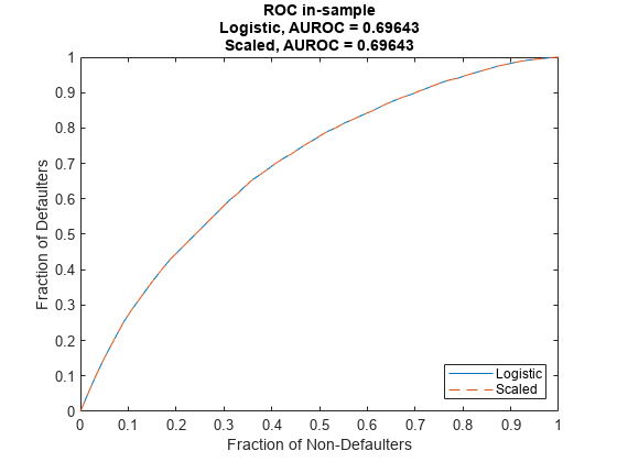
Discrimination measures only ranking of customers, that is, whether riskier customers get assigned higher PDs than less risky customers. Therefore, if you scale the probabilities or apply another monotonic transformation that results in valid probabilities, the AUROC measure does not change.

For example, multiply the predicted PDs by a factor of 2, which preserves the ranking (where the worse customers have higher PDs). To compare the results, pass the modified PDs as reference PDs.

PD0 = predict(pdModel,data);
PD1 = 2*PD0;

disp([PD0(1:10) PD1(1:10)])

    0.0090    0.0181
    0.0052    0.0104
    0.0044    0.0088
    0.0038    0.0076
    0.0035    0.0071
    0.0036    0.0072
    0.0019    0.0037
    0.0011    0.0022
    0.0164    0.0328
    0.0094    0.0189

Verify that the discrimination measure is not affected using modelDiscriminationPlot.

modelDiscriminationPlot(pdModel,data,'DataID','in-sample','ReferencePD',PD1,'ReferenceID','Scaled')

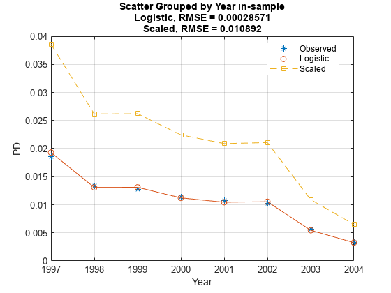
Use modelCalibrationPlot to visualize the observed default rates compared to the predicted probabilities of default (PD). The calibration, however, is severely affected by the change. The modified PDs are far away from the observed default rates and the RMSE for the modified PDs is orders of magnitude higher than the RMSE of the original PDs.

modelCalibrationPlot(pdModel,data,'Year',"DataID",'in-sample','ReferencePD',PD1,"ReferenceID",'Scaled')

Same Calibration, Different Discrimination

On the other hand, you can also modify the predicted PDs to keep the calibration metric unchanged and worsen the discrimination metric.

One way to do this is to permute the PDs within a group. By doing this, the ranking within each group is affected, but the average PD for the group is unchanged.

rng('default'); % for reproducibility
PD1 = PD0;
for Year=1997:2004
   Ind = data.Year==Year;
   PDYear = PD0(Ind);
   PD1(Ind) = PDYear(randperm(length(PDYear)));
end

Verify that the discrimination measure is worse for the modified PDs using modelDiscriminationPlot.

modelDiscriminationPlot(pdModel,data,'DataID','in-sample','ReferencePD',PD1,'ReferenceID','Permutation')

The modelCalibrationPlot function measures model calibration for PDs on grouped data. As long as the average PD for the group is unchanged, the reported calibration using the same grouping variable does not change.

modelCalibrationPlot(pdModel,data,'Year',"DataID",'in-sample','ReferencePD',PD1,"ReferenceID",'Permutation')

This example shows that discrimination and calibration metrics do not necessarily go hand in hand. Different predictions may have similar RMSE but much different AUROC, or similar AUROC but much different RMSE. Therefore, it is important to look at both discrimination and calibration as part of a model validation framework.

References

[1] Baesens, Bart, Daniel Roesch, and Harald Scheule. Credit Risk Analytics: Measurement Techniques, Applications, and Examples in SAS. Wiley, 2016.

[2] Basel Committee on Banking Supervision, "Studies on the Validation of Internal Rating Systems", Working Paper No. 14, 2005.