Main Content

inverseKinematics

Create inverse kinematic solver

Description

The inverseKinematics System object™ creates an inverse kinematic (IK) solver to calculate joint configurations for a desired end-effector pose based on a specified rigid body tree model. Create a rigid body tree model for your robot using the rigidBodyTree class. This model defines all the joint constraints that the solver enforces. If a solution is possible, the joint limits specified in the robot model are obeyed.

To specify more constraints besides the end-effector pose, including aiming constraints, position bounds, or orientation targets, consider using generalizedInverseKinematics. This object allows you to compute multiconstraint IK solutions.

For closed-form analytical IK solutions, see analyticalInverseKinematics.

To compute joint configurations for a desired end-effector pose:

  1. Create the inverseKinematics object and set its properties.

  2. Call the object with arguments, as if it were a function.

To learn more about how System objects work, see What Are System Objects?

Creation

Description

ik = inverseKinematics creates an inverse kinematic solver. To use the solver, specify a rigid body tree model in the RigidBodyTree property.

example

ik = inverseKinematics(Name,Value) creates an inverse kinematic solver with additional options specified by one or more Name,Value pair arguments. Name is a property name and Value is the corresponding value. Name must appear inside single quotes (''). You can specify several name-value pair arguments in any order as Name1,Value1,...,NameN,ValueN.

Properties

expand all

Unless otherwise indicated, properties are nontunable, which means you cannot change their values after calling the object. Objects lock when you call them, and the release function unlocks them.

If a property is tunable, you can change its value at any time.

For more information on changing property values, see System Design in MATLAB Using System Objects.

Rigid body tree model, specified as a rigidBodyTree object. If you modify your rigid body tree model, reassign the rigid body tree to this property. For example:

Create IK solver and specify the rigid body tree.

ik = inverseKinematics('RigidBodyTree',rigidbodytree)

Modify the rigid body tree model.

addBody(rigidbodytree,rigidBody('body1'),'base')

Reassign the rigid body tree to the IK solver. If the solver or the step function is called before modifying the rigid body tree model, use release to allow the property to be changed.

ik.RigidBodyTree = rigidbodytree;

Algorithm for solving inverse kinematics, specified as either 'BFGSGradientProjection' or 'LevenbergMarquardt'. For details of each algorithm, see Inverse Kinematics Algorithms.

Parameters associated with the specified algorithm, specified as a structure. The fields in the structure are specific to the algorithm. See Solver Parameters.

Usage

Description

[configSol,solInfo] = ik(endeffector,pose,weights,initialguess) finds a joint configuration that achieves the specified end-effector pose. Specify an initial guess for the configuration and your desired weights on the tolerances for the six components of pose. Solution information related to execution of the algorithm, solInfo, is returned with the joint configuration solution, configSol.

example

Input Arguments

expand all

End-effector name, specified as a character vector. The end effector must be a body on the rigidBodyTree object specified in the inverseKinematics System object.

End-effector pose, specified as a 4-by-4 homogeneous transform. This transform defines the desired position and orientation of the rigid body specified in the endeffector property.

Weight for pose tolerances, specified as a six-element vector. The first three elements correspond to the weights on the error in orientation for the desired pose. The last three elements correspond to the weights on the error in xyz position for the desired pose.

Initial guess of robot configuration, specified as a structure array or vector. Use this initial guess to help guide the solver to a desired robot configuration. The solution is not guaranteed to be close to this initial guess.

To use the vector form, set the DataFormat property of the object assigned in the RigidBodyTree property to either 'row' or 'column'.

Output Arguments

expand all

Robot configuration, returned as a structure array. The structure array contains these fields:

  • JointName — Character vector for the name of the joint specified in the RigidBodyTree robot model

  • JointPosition — Position of the corresponding joint

This joint configuration is the computed solution that achieves the desired end-effector pose within the solution tolerance.

Note

For revolute joints, if the joint limits exceed a range of 2*pi, where joint position wrapping occurs, then the returned joint position is the one closest to the joint's lower bound.

To use the vector form, set the DataFormat property of the object assigned in the RigidBodyTree property to either 'row' or 'column'.

Solution information, returned as a structure. The solution information structure contains these fields:

  • Iterations — Number of iterations run by the algorithm.

  • NumRandomRestarts — Number of random restarts because algorithm got stuck in a local minimum.

  • PoseErrorNorm — The magnitude of the pose error for the solution compared to the desired end-effector pose.

  • ExitFlag — Code that gives more details on the algorithm execution and what caused it to return. For the exit flags of each algorithm type, see Exit Flags.

  • Status — Character vector describing whether the solution is within the tolerance ('success') or the best possible solution the algorithm could find ('best available').

Object Functions

To use an object function, specify the System object as the first input argument. For example, to release system resources of a System object named obj, use this syntax:

release(obj)

expand all

stepRun System object algorithm
releaseRelease resources and allow changes to System object property values and input characteristics
resetReset internal states of System object

Examples

collapse all

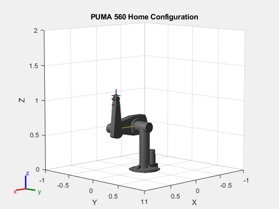
Load a PUMA 560 manipulator from the Robotics System Toolbox™ loadrobot and show the robot model in a figure.

puma = loadrobot("puma560");
show(puma,homeConfiguration(puma),PreservePlot=false);
axis([-1 1 -1 1 0 2])
title("PUMA 560 Home Configuration")

Figure contains an axes object. The axes object with title PUMA 560 Home Configuration, xlabel X, ylabel Y contains 20 objects of type patch, line. These objects represent link1, link2, link3, link4, link5, link6, link7, link2_mesh, link3_mesh, link4_mesh, link5_mesh, link6_mesh, link7_mesh, link1_mesh.

The desired position for the end effector of the robot to reach is [-0.5 0.5 0.75]. Inverse Kinematics uses a desired pose to solve for joint configurations, so first convert the position into an SE(3) homogeneous transformation matrix with the desired translation. Then plot the pose transformation.

pos = [-0.5 0.5 0.75];
poseTF = trvec2tform(pos);
hold on
plotTransforms(pos,eul2quat([0 0 0]),FrameSize=0.2);
title("PUMA 560 and End-Effector Target Position")

Figure contains an axes object. The axes object with title PUMA 560 and End-Effector Target Position, xlabel X, ylabel Y contains 24 objects of type patch, line. These objects represent link1, link2, link3, link4, link5, link6, link7, link2_mesh, link3_mesh, link4_mesh, link5_mesh, link6_mesh, link7_mesh, link1_mesh.

Create an inverseKinematics System object™ for the puma robot model. Specify weights for the rotation and the position of the pose. Because the goal is for the end-effector to reach that position with no constraint on orientation, set orientation-angle weights to zero so that the orientation solution does not matter to the IK solver. Use the home configuration of the robot as an initial guess.

ik = inverseKinematics("RigidBodyTree",puma);
weights = [0 0 0 1 1 1];
initialguess = homeConfiguration(puma);

Calculate the joint positions using the ik System object. Use the last link in the robot model, link7, as the end effector.

[configSoln,solnInfo] = ik("link7",poseTF,weights,initialguess);

Show the generated solution configuration, which now reaches the goal position.

show(puma,configSoln,PreservePlot=false);
title("End-Effector Target Position Achieved")

Figure contains an axes object. The axes object with title End-Effector Target Position Achieved, xlabel X, ylabel Y contains 24 objects of type patch, line. These objects represent link1, link2, link3, link4, link5, link6, link7, link2_mesh, link3_mesh, link4_mesh, link5_mesh, link6_mesh, link7_mesh, link1_mesh.

Note that for most IK problems, there are multiple configurations that can reach the desired pose target. Because the solver is optimization-based, the solver could approach a solution that does not actually reach the desired pose. If this occurs, the solver automatically restarts and uses a random configuration as the initial guess. This means that running the function more than once for the same pose target could yield different configurations that all reach the pose target. To avoid randomness, you can either set the random number generator seed or you can use an initial guess that is closer to the solution while also disabling AllowRandomRestart.

ik.SolverParameters.AllowRandomRestart = false

If you must find all possible solutions, use the analyticalInverseKinematics object.

References

[1] Badreddine, Hassan, Stefan Vandewalle, and Johan Meyers. "Sequential Quadratic Programming (SQP) for Optimal Control in Direct Numerical Simulation of Turbulent Flow." Journal of Computational Physics. 256 (2014): 1–16. doi:10.1016/j.jcp.2013.08.044.

[2] Bertsekas, Dimitri P. Nonlinear Programming. Belmont, MA: Athena Scientific, 1999.

[3] Goldfarb, Donald. "Extension of Davidon’s Variable Metric Method to Maximization Under Linear Inequality and Equality Constraints." SIAM Journal on Applied Mathematics. Vol. 17, No. 4 (1969): 739–64. doi:10.1137/0117067.

[4] Nocedal, Jorge, and Stephen Wright. Numerical Optimization. New York, NY: Springer, 2006.

[5] Sugihara, Tomomichi. "Solvability-Unconcerned Inverse Kinematics by the Levenberg–Marquardt Method." IEEE Transactions on Robotics Vol. 27, No. 5 (2011): 984–91. doi:10.1109/tro.2011.2148230.

[6] Zhao, Jianmin, and Norman I. Badler. "Inverse Kinematics Positioning Using Nonlinear Programming for Highly Articulated Figures." ACM Transactions on Graphics Vol. 13, No. 4 (1994): 313–36. doi:10.1145/195826.195827.
Extended Capabilities

Version History

Introduced in R2016b

expand all