Inverse Kinematics
Compute joint configurations to achieve an end-effector pose
Libraries:
Robotics System Toolbox /
Manipulator Algorithms
Description
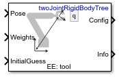
The Inverse Kinematics block uses an inverse kinematic (IK) solver to
calculate joint configurations for a desired end-effector pose based on a specified rigid body
tree model. Create a rigid body tree model for your robot using the rigidBodyTree class. The rigid body tree model defines all the joint constraints
that the solver enforces.
Specify the RigidBodyTree parameter and the desired end effector inside
the block mask. You can also tune the algorithm parameters in the Solver
Parameters tab.
Input the desired end-effector Pose, the Weights on pose tolerance, and an InitialGuess for the joint configuration. The solver outputs a robot configuration, Config, that satisfies the end-effector pose within the tolerances specified in the Solver Parameters tab.
Examples
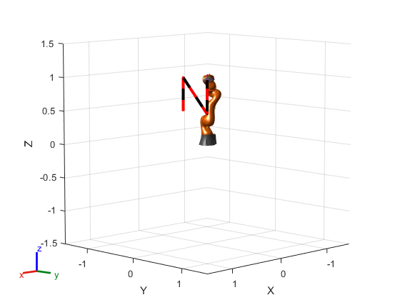
Trace an End-Effector Trajectory with Inverse Kinematics in Simulink
Compute inverse kinematics in Simulink® to trace a defined end-effector trajectory with a rigid body robot model.
Ports
Input
Output
Parameters
References
[1] Badreddine, Hassan, Stefan Vandewalle, and Johan Meyers. "Sequential Quadratic Programming (SQP) for Optimal Control in Direct Numerical Simulation of Turbulent Flow." Journal of Computational Physics. 256 (2014): 1–16. doi:10.1016/j.jcp.2013.08.044.
[2] Bertsekas, Dimitri P. Nonlinear Programming. Belmont, MA: Athena Scientific, 1999.
[3] Goldfarb, Donald. "Extension of Davidon’s Variable Metric Method to Maximization Under Linear Inequality and Equality Constraints." SIAM Journal on Applied Mathematics. Vol. 17, No. 4 (1969): 739–64. doi:10.1137/0117067.
[4] Nocedal, Jorge, and Stephen Wright. Numerical Optimization. New York, NY: Springer, 2006.
[5] Sugihara, Tomomichi. "Solvability-Unconcerned Inverse Kinematics by the Levenberg–Marquardt Method." IEEE Transactions on Robotics. Vol. 27, No. 5 (2011): 984–91. doi:10.1109/tro.2011.2148230.
[6] Zhao, Jianmin, and Norman I. Badler. "Inverse Kinematics Positioning Using Nonlinear Programming for Highly Articulated Figures." ACM Transactions on Graphics. Vol. 13, No. 4 (1994): 313–36. doi:10.1145/195826.195827.