Main Content

trapveltraj

Generate trajectories with trapezoidal velocity profiles

Description

example

[q,qd,qdd,tSamples,pp] = trapveltraj(wayPoints,numSamples) generates a trajectory through a given set of input waypoints that follow a trapezoidal velocity profile. The function outputs positions, velocities, and accelerations at the given time samples, tSamples, based on the specified number of samples, numSamples. The function also returns the piecewise polynomial pp form of the polynomial trajectory with respect to time.

[q,qd,qdd,tSamples,pp] = trapveltraj(wayPoints,numSamples,Name,Value) specifies additional parameters using Name,Value pair arguments.

Examples

collapse all

Use the trapveltraj function with a given set of 2-D xy waypoints.

wpts = [0 45 15 90 45; 90 45 -45 15 90];

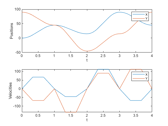
Compute the trajectory for a given number of samples (501). The function outputs the trajectory positions (q), velocity (qd), acceleration (qdd), time vector (tvec), and polynomial coefficients (pp) of the polynomial that achieves the waypoints using trapezoidal velocities.

[q,qd,qdd,tvec,pp] = trapveltraj(wpts,501);

Plot the trajectories for the x- and y-positions and the trapezoidal velocity profile between each waypoint.

subplot(2,1,1)
plot(tvec, q)
xlabel('t')
ylabel('Positions')
legend('X','Y')
subplot(2,1,2)
plot(tvec, qd)
xlabel('t')
ylabel('Velocities')
legend('X','Y')

You can also verify the actual positions in the 2-D plane. Plot the separate rows of the q vector and the waypoints as x- and y-positions.

figure
plot(q(1,:),q(2,:),'-b',wpts(1,:),wpts(2,:),'or')

Input Arguments

collapse all

Points for waypoints of trajectory, specified as an n-by-p matrix, where n is the dimension of the trajectory and p is the number of waypoints.

Example: [1 4 4 3 -2 0; 0 1 2 4 3 1]

Data Types: single | double

Number of samples in output trajectory, specified as a positive integer.

Data Types: single | double

Name-Value Arguments

Specify optional pairs of arguments as Name1=Value1,...,NameN=ValueN, where Name is the argument name and Value is the corresponding value. Name-value arguments must appear after other arguments, but the order of the pairs does not matter.

Before R2021a, use commas to separate each name and value, and enclose Name in quotes.

Example: 'PeakVelocity',5

Note

Due to the nature of the trapezoidal velocity profile, you can only set at most two of the following parameters.

Peak velocity of the profile segment, specified as the comma-separated pair consisting of 'PeakVelocity' and a scalar, vector, or matrix. This peak velocity is the highest velocity achieved during the trapezoidal velocity profile.

A scalar value is applied to all elements of the trajectory and between all waypoints. An n-element vector is applied to each element of the trajectory between all waypoints. An n-by-(p–1) matrix is applied to each element of the trajectory for each waypoint.

Data Types: single | double

Acceleration of the velocity profile, specified as the comma-separated pair consisting of 'Acceleration' and a scalar, vector, or matrix. This acceleration defines the constant acceleration from zero velocity to the PeakVelocity value.

A scalar value is applied to all elements of the trajectory and between all waypoints. An n-element vector is applied to each element of the trajectory between all waypoints. An n-by-(p–1) matrix is applied to each element of the trajectory for each waypoint.

Data Types: single | double

Duration of each of the p–1 trajectory segments, specified as the comma-separated pair consisting of 'EndTime' and a scalar, vector, or matrix.

A scalar value is applied to all elements of the trajectory and between all waypoints. An n-element vector is applied to each element of the trajectory between all waypoints. An n-by-(p–1) matrix is applied to each element of the trajectory for each waypoint.

Data Types: single | double

Duration of acceleration phase of velocity profile, specified as the comma-separated pair consisting of 'AccelTime' and a scalar, vector, or matrix.

A scalar value is applied to all elements of the trajectory and between all waypoints. An n-element vector is applied to each element of the trajectory between all waypoints. An n-by-(p–1) matrix is applied to each element of the trajectory for each waypoint.

Data Types: single | double

Output Arguments

collapse all

Positions of the trajectory at the given time samples in tSamples, returned as n-by-m matrix, where n is the dimension of the trajectory, and m is equal to numSamples.

Data Types: single | double

Velocities of the trajectory at the given time samples in tSamples, returned as n-by-m matrix, where n is the dimension of the trajectory, and m is equal to numSamples.

Data Types: single | double

Accelerations of the trajectory at the given time samples in tSamples, returned as n-by-m matrix, where n is the dimension of the trajectory, and m is equal to numSamples.

Data Types: single | double

Time samples for the trajectory, returned as an m-element vector. The output position, q, velocity, qd, and accelerations, qdd are sampled at these time intervals.

Example: 0:0.01:10

Data Types: single | double

Piecewise polynomials, returned as a cell array of structures that defines the polynomial for each section of the piecewise trajectory. If all the elements of the trajectory share the same breaks, the cell array is a single piecewise polynomial structure. Otherwise, the cell array has n elements, which correspond to each of the different trajectory elements (dimensions). Each structure contains the fields:

  • form: 'pp'.

  • breaks: p-element vector of times when the piecewise trajectory changes forms. p is the number of waypoints.

  • coefs: n(p–1)-by-order matrix for the coefficients for the polynomials. n(p–1) is the dimension of the trajectory times the number of pieces. Each set of n rows defines the coefficients for the polynomial that described each variable trajectory.

  • pieces: p–1. The number of breaks minus 1.

  • order: Degree of the polynomial + 1. For example, cubic polynomials have an order of 4.

  • dim: n. The dimension of the control point positions.

You can build your own piecewise polynomials using mkpp, or evaluate the polynomial at specified times using ppval.

Piecewise-polynomial, returned as a structure that defines the polynomial for each section of the piecewise trajectory. You can build your own piecewise polynomials using mkpp, or evaluate the polynomial at specified times using ppval. The structure contains the fields:

  • form: 'pp'.

  • breaks: p-element vector of times when the piecewise trajectory changes forms. p is the number of waypoints.

  • coefs: n(p–1)-by-order matrix for the coefficients for the polynomials. n(p–1) is the dimension of the trajectory times the number of pieces. Each set of n rows defines the coefficients for the polynomial that described each variable trajectory.

  • pieces: p–1. The number of breaks minus 1.

  • order: Degree of the polynomial + 1. For example, cubic polynomials have an order of 4.

  • dim: n. The dimension of the control point positions.

References

[1] Lynch, Kevin M., and Frank C. Park. Modern Robotics: Mechanics, Planning and Control. Cambridge: Cambridge University Press, 2017.

[2] Spong, Mark W., Seth Hutchinson, and M. Vidyasagar. Robot Modeling and Control. John Wiley & Sons, 2006.

Extended Capabilities

C/C++ Code Generation
Generate C and C++ code using MATLAB® Coder™.

Version History

Introduced in R2019a