Plan Path of Robotic Arm Mounted on Quadrotor

Create UAV as Floating Base

First, create an empty rigid body tree and a rigid body with a floating joint.

uavWithArm = rigidBodyTree(DataFormat="row");
uav = rigidBody("uav");
uav.Joint = rigidBodyJoint("uav_base_floating_joint","floating");

Get the geometry of a quadrotor UAV as a triangulation object by reading from the multirotor STL file.

tr = stlread("multirotor.stl");

Scale the geometry so that the dimensions are more accurate to the size of a real quadrotor UAV.

scaledtr = triangulation(tr.ConnectivityList,tr.Points/200);
trimesh(scaledtr);
title("UAV Triangulation")
xlabel("X (m)")
ylabel("Y (m)")
zlabel("Z (m)")
axis equal

[az,el] = view;

Notice that the collision geometry is nonconvex. To accurately model this geometry for collision checking, use the collisionVHACD function to decompose this into a composite of approximate convex meshes.

options = vhacdOptions("IndividualMesh",MaxNumConvexHulls=8,MaxNumVerticesPerHull=50);
compositeMeshes = collisionVHACD(scaledtr,options);

Add each of the decomposed meshes to the rigid body using addCollision.

for i = 1:length(compositeMeshes)
    addCollision(uav,compositeMeshes{i});
end

Add the UAV rigid body to the floating-base rigid body tree and visualize the UAV.

addBody(uavWithArm,uav,uavWithArm.BaseName);
show(uavWithArm,Collisions="on");
title("UAV Collision Mesh")
axis equal
xlabel("X (m)")
ylabel("Y (m)")
zlabel("Z (m)")
view([az,el])

Mount Robotic Arm on UAV

Load the rigid body tree for the Open Manipulator robotic arm from Robotis.

openmanip = loadrobot("robotisOpenManipulator",DataFormat="row");

To mount to the robotic arm on the underside of the UAV, set the fixed transform of the first body of the arm that rotates the arm pi radians in the y-axis and applies a small z-axis translation offset. The z-axis offset is to avoid self-collisions. Alternatively, one can specify the SkippedSelfCollisions property of the planner with the link pair to be ignored while self-collision checking. See example Skip Self-Collision Checking Between Specific Body Pairs for more details.

fixedTF = eul2tform([0 pi 0])*trvec2tform([0 0 1e-4]);
setFixedTransform(openmanip.Bodies{1}.Joint,fixedTF);

Mount the robotic arm rigid body tree model to the UAV floating base and visualize the UAV with the mounted arm.

addSubtree(uavWithArm,"uav",openmanip);
show(uavWithArm,Collisions="on",Frames="off");
title("UAV With Mounted Robotic Arm")
axis equal
xlabel("X (m)")
ylabel("Y (m)")
zlabel("Z (m)")
view(225,15)

Motion Planning Problem

The motion planning problem is to find a collision free path from a starting joint configuration to a desired goal configuration. To do this, you must define these aspects of the problem:

Starting and Goal Joint Configurations

The joint configuration of the UAV represents the pose of the UAV in the world. Thus, define the configuration vector of the UAV to describe its pose in the world is given as $\left[{\mathit{q}}_{\mathrm{uav}}{\mathit{t}}_{\mathrm{uav}}{\mathit{q}}_{\mathrm{robotic}\mathrm{arm}}\right]$ where,

Set the starting configuration with the floating body "uav" at the xyz-coordinate [0 0 -1] and -pi/3 rad for the third joint on the arm.

qstart = homeConfiguration(uavWithArm);
qstart(5:7) = [0 0 -1];
qstart(end-3) = -pi/3;

Use the start configuration and modify it to get a goal configuration. Set the goal configuration of the body "uav" to the xyz-coordinate [2 0 2] at an orientation of [pi/2 0 0] Euler ZYX.

qgoal = qstart;
qgoal(5:7) = [2 0 2];
qgoal(1:4) = eul2quat([pi/2 0 0]);

Add Obstacles in Environment

Create an environment using collision boxes and set the positions of the boxes such that they create a wall between the start and goal configurations.

env={collisionBox(0.5,4,3,Pose=trvec2tform([1.0 0.0 -1.3])),...
     collisionBox(0.5,4,1.5,Pose=trvec2tform([1.0 0.0 1.8]))};

Visualize the planning problem. Show the collision geometries and hide the frames on the UAV.

figure
show(uavWithArm,qstart,Collisions="on",Frames="off");
hold on
showCollisionArray(env);
show(uavWithArm,qgoal,Collisions="on",Frames="off");
title("Planning Problem")
view(0,0)
hold off

Robot's Kinematic Constraints

In this example, set the translational PositionLimits of the floating joint associated with the "uav" rigidBody such that it is constrained to fly within cartesian bounds (say a physical safety cage) of [-1,3] in X, [-2,2] in Y, and [-2.5,2.5] in Z, of the workspace's frame. Note that the rotational limits of a floating rigidBodyJoint cannot be set and are NaNs.

uavBody=getBody(uavWithArm,"uav");
uavBody.Joint.PositionLimits(5:end,:)=[-1,3;-2,2;-2.5,2.5];

Find Collision Free Path

Find a collision free path between the start and goal joint configuration. To find such a path, this example uses manipulatorRRT to plan a geometric collision-free path.

rrt = manipulatorRRT(uavWithArm,env, ...
    MaxConnectionDistance=0.5, ...
    ValidationDistance=0.1, ...
    SkippedSelfCollisions="parent");

Seed the random number generator and plan a path using RRT, shorten the output plan and interpolate the shortened path to make it smoother.

rng(0,"twister");
plannedpath = plan(rrt,qstart,qgoal);
shortenedPath = shorten(rrt,plannedpath,40);
rrtpath = interpolate(rrt,shortenedPath,10);

Visualize Planned Path

Visualize the planned geometric path of UAV with a mounted robotic arm as an animation.

show(uavWithArm,qstart,Collisions="on");
title("UAV Flight Animation")
view(0,0)
hold on
plot3(rrtpath(:,5),rrtpath(:,6),rrtpath(:,7),"k-",LineWidth=1)
showCollisionArray(env);
rc = rateControl(10);
for i = 1:1:size(rrtpath,1)
    show(uavWithArm,rrtpath(i,:),...
        PreservePlot=false,...
        FastUpdate=true, ...
        Frames="off", ...
        Collisions="on");
    waitfor(rc);
    view(0,0)
end
hold off

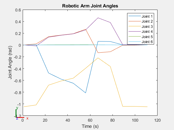
Note that the arm also moves along the path to avoid colliding with the obstacles in the environment. Plot the joint angles of the robotic arm in the planned path.

plot(rrtpath(:,8:end),"-")
title("Robotic Arm Joint Angles")
xlabel("Time (s)")
ylabel("Joint Angle (rad)")
legend("Joint "+string(1:6))

Next Steps

Adding Constraints to Motion Plan

Notice how the planned geometric path doesn't impose any orientation restrictions on the UAV nor do the interpolated states impose kinematic constraints to achieve a feasible trajectory. In order to add such kinematic constraints to the geometric path, use a custom nav.StateSpace derived from a manipulatorStateSpace. Refer to Plan Paths With End-Effector Constraints Using State Spaces For Manipulators Documentation example as a reference.

Copyrights The MathWorks, Inc. 2023