Correlate an IBIS Model Against Its Source SPICE Model
R2026bUse this topic to verify the accuracy of a generated IBIS model by comparing its transient waveforms against the original transistor-level SPICE model. You set up paired "golden waveform" simulation decks: one uses your SPICE subcircuit, and the other uses the IBIS file through HSPICE's B-element. You run both through the same channel topology, then use a MATLAB script to overlay the results and compute quantitative correlation metrics.
Why Correlation Matters
An IBIS model is a behavioral abstraction. The conversion from transistor-level SPICE to IBIS discards information: device physics reduce to piecewise-linear IV tables, continuous transient behavior becomes sampled VT waveform points, and frequency-dependent parasitics collapse into a single C_comp value. Your IBIS file may pass ibischk with zero errors and still produce waveforms that diverge from the original SPICE model in a realistic channel.
Correlation is the only way to confirm that your IBIS model is accurate enough for signal integrity analysis. Without it, you trust that the extraction process preserved the electrical behavior that matters (timing margins, voltage overshoot, ringback settling, and impedance matching) without ever verifying it directly.
An uncorrelated IBIS model can create silent errors:
Over-designed systems: If the IBIS model predicts worse overshoot than the real silicon, board designers add unnecessary termination components. This increases BOM cost and board area.
Under-designed systems: If the IBIS model predicts better timing margins than reality, the design passes simulation but fails in hardware. You discover the problem only at silicon validation, when changes are expensive.
Misattributed failures: When a system-level simulation shows a marginal eye diagram, engineers cannot tell whether the problem is the model or the channel. You need correlation data to establish confidence in the model.
Important Note: The same parameter values (such as rout, odt, cpad, and vdd) must be used in both the characterization decks and the golden correlation decks. A mismatch here (e.g., using rout=34 in generation but rout=50 in correlation) will produce false correlation failures.
What This Topic Covers
This topic walks you through a complete SPICE-to-IBIS correlation workflow:
Correlation topology. You build a test circuit with a transmission line and capacitive load that produces realistic reflections. This exercises both the driver's switching behavior and the clamp structures.
Paired simulation. You simulate the same topology twice: once with the original SPICE model ("spice"), and once with the generated IBIS model ("ibis") through HSPICE's B-element.
Waveform comparison. A MATLAB script reads the simulation outputs and overlays three waveforms: SPICE (reference), IBIS with VT waveform data, and IBIS with Ramp data only.
Accuracy assessment. Quantitative metrics (peak error, RMS error) tell you whether the model is accurate enough for your application.
The comparison between IBIS-VT and IBIS-Ramp is instructive. The Ramp-only model uses only the dV/dt_r and dV/dt_f values from the IBIS file. This is a coarse linear approximation of the switching edge. The VT model uses the full [Rising Waveform] and [Falling Waveform] tables, which capture the actual edge shape including the initial launch, mid-swing behavior, and final settling. When you see the difference between these two in the correlation plot, it demonstrates why VT waveform data is essential for accurate signal integrity simulation.
Prerequisites
Before you run this workflow, make sure you have:
HSPICE. Both the SPICE and IBIS golden decks are run in HSPICE. The IBIS decks specifically require HSPICE's B-element IBIS simulator.
MATLAB R2026b or later. The correlation script uses string arrays and the
readtableVariableNamingRule="preserve"option. R2026b is the minimum supported release.Mixed-Signal Blockset. The script converts HSPICE binary
.tr0files to CSV withtr0Reader(and its companionssw0Reader/ac0Reader), which ship with Mixed-Signal Blockset. This is a separately licensed toolbox.A generated
.ibsfile. The IBIS decks referencefile='your_model.ibs'. You produce this by completing the Generate HSPICE Simulation Decks for IBIS Characterization and Create IBIS Model from SPICE Simulation Data workflows first. No sample.ibsships with this topic.
No Mixed-Signal Blockset? You can skip tr0Reader entirely and read ASCII output instead. Add .options post_version=2001 (or use .print tran) to your decks so HSPICE writes an ASCII .tr0/.printfile, then comment out the tr0Reader calls in the conversion section below and point readtable directly at the ASCII file with appropriate format options. The rest of the script is unchanged.
Workflow: From IBIS Model to Validated Correlation
Follow these seven steps to run a complete correlation. The sections below provide detail and reference decks for each step.
Generate your IBIS model. Use the IBIS Designer SPICE Simulation workflow to produce the
.ibsfile you want to validate (see Create IBIS Model from SPICE Simulation Data).Choose deck pairs. Choose the SPICE and IBIS deck pair for your model type and signaling mode from the "Reference Deck Files" table below.
Customize the decks. In the SPICE deck, update the
.includepath and subcircuit name to point at your buffer model. In the IBIS deck, set thefile=andmodel=parameters to your generated.ibsfile.Create corner variants. Duplicate each typical-corner deck for slow and fast corners. In SPICE decks, change
.tempand.param vdd. In IBIS decks, change thetyp=parameter (typ,min, ormax).Run paired simulations. Execute all decks in HSPICE (6 simulations for a 3-corner I/O model: 3 SPICE + 3 IBIS). Verify convergence before you continue.
Compare waveforms. Use the MATLAB script below to overlay the SPICE reference against the IBIS-VT and IBIS-Ramp results. Compute quantitative error metrics.
Assess accuracy. If VT peak error is < 5% of Vdd, your model is ready for distribution. If not, investigate the extraction (see "Interpreting Correlation Results" below) and iterate.
Correlation Circuit Topologies
The correlation circuits stress-test the IBIS model in conditions where behavioral accuracy matters most. A simple resistive load exercises only the steady-state IV curves. Instead, the circuits include a transmission line that creates impedance discontinuities and produces reflections. These reflections swing the pad voltage beyond the supply rails, turning on the clamp structures. Clamp structures are the hardest part of the IBIS model to get right.
Driver Correlation Circuit
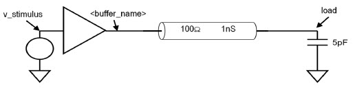
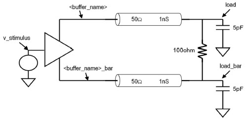
The driver circuit places the buffer under test at one end of a lossy channel and probes the voltage at the far-end load. The channel impedance is intentionally mismatched against the driver, creating reflections at the buffer pad that exercise the power and ground clamp structures. The 5 pF capacitive load represents a realistic receiver input (die capacitance + PCB pad).
The single-ended and differential decks realize this idea with different channels:
Single-ended: one 100-ohm transmission line, mismatched against a typical 30-50 ohm driver impedance, with a 5 pF far-end load. You compare waveforms at the far-end voltage
v(load).Differential: two 50-ohm transmission lines (one per leg) with a 100-ohm differential termination across the load pair and a 5 pF load on each leg. You compare the differential far-end voltage
v(load,load_n).
Single-ended driver correlation topology: buffer drives into mismatched T-line with capacitive far-end load:
Differential driver correlation topology: each leg drives a 50-ohm line into a 100-ohm differential termination:
Receiver Correlation Circuit
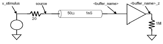
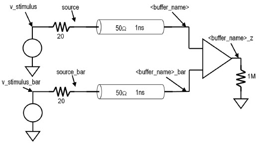
The receiver circuit drives the buffer pad through a channel that produces reflections from the impedance mismatch at the receiver. The piecewise linear (PWL) source swings the full 0-to-Vdd range with realistic edge rates. The series resistor (20 ohm) combined with the 50-ohm line creates a source impedance mismatch. This mismatch produces reflections at the receiver pad that exercise the receiver's termination (ODT) and clamp behavior. You compare waveforms at v(pad) at the buffer input.
Single-ended receiver correlation topology: source-terminated line drives buffer pad with reflections:
Differential receiver correlation topology:
HSPICE B-Element: Simulating IBIS Models in SPICE
The "ibis" decks use HSPICE's built-in IBIS simulator through the B-element syntax. You run the IBIS model in the same SPICE environment with the same stimulus and channel. The only difference is the buffer model.
Bbufname vdd vss pad stimulus enable corein vdd vss
+ file='path/to/model.ibs'
+ model='model_name'
+ power=off typ=typ ramp_fwf=2 ramp_rwf=2
The form above is for an I/O model; the terminal list and continuation lines differ for Output and Input models; see Match the Deck to the Model Type below.
Key parameters:
file: path to the IBIS filemodel: model name in the IBIS filetyp=typ: selects the typical corner column from the IBIS tables (usetyp=minortyp=maxfor corner correlation)ramp_fwf=2, ramp_rwf=2: use VT waveform data for both falling and rising edges (0 = Ramp only, 2 = VT waveforms)power=off: disable internal power rail modeling (the deck uses external supplies instead)
The VT-versus-Ramp comparison only applies to the driver switching edge, so it is only meaningful for models that carry driver waveform data: Output and I/O models. Input models contain no [Ramp] or [Rising Waveform] / [Falling Waveform] tables, so there is nothing to compare. For that reason only the driver decks instantiate the IBIS model twice, to compare VT-based accuracy against Ramp-only accuracy:
VT instance (
ramp_fwf=2): Uses the full[Rising Waveform]/[Falling Waveform]tables. Its far-end probe reuses the SPICE deck'sv(load)node name so the two waveforms overlay directly; in SiViewer, selecting the SPICE and IBIS decks together plots the shared node for a single-click overlay.Ramp instance (
ramp_fwf=0): Uses onlydV/dt_randdV/dt_f, probed asv(load_ramp).
A receiver deck exercises the buffer in input mode, where no switching edge is generated, so it instantiates the model just once (a single B-element for single-ended, one per pad for differential) as a VT instance with no Ramp instance. \
Match the Deck to the Model Type
Each *_ibis.spi deck is written for a specific Model_type and must be run against an IBIS file whose [Model] is that same type: I/O with I/O, Output with Output, Input with Input. The B-element's terminal list differs by type, and a mismatch aborts the simulation rather than producing a wrong-but-runnable result:
| B-element terminals | Power-reference line ( |
|
|---|---|---|---|
I/O |
| required | required (driver edges) |
Output |
| required | required (driver edges) |
Input |
| omitted | omitted |
An Input model carries no [Ramp] or waveform tables, so an Input B-element takes exactly four nodes (vddq, vssq, the pad, and the receiver decision output) with no power-reference continuation line and no ramp flags. Supplying the I/O six-node form to an Input model aborts with Incorrect number of nodes specified for input buffer, expecting 4 nodes. Conversely, feeding an I/O or Output model into an Input-style deck (or an I/O model into an Output-only deck) produces a Voltage loop at the node of out_of_in abort, because the receiver path the model expects has nowhere to connect. If you only have an I/O model, use the I/O decks; the Output-only and Input-only decks require models of those exact types.
Note for Spectre users: The B-element is HSPICE-specific, but only the IBIS deck depends on it. The SPICE decks use standard subcircuit netlists and a common testbench topology, so they port to other simulators with only mechanical changes: the output and analysis statements (.probe, .options post) and the PWL source syntax need adjusting for Spectre, but the circuit and comparison methodology are unchanged. In Spectre, the equivalent to the B-element is the ibis_buffer cell in Cadence's IBIS-to-SPICE flow; the topology, probe names, and comparison methodology remain the same, and only the IBIS instantiation syntax differs. Consult your Spectre documentation for the equivalent parameter mapping.
Reference Deck Files
This topic provides 16 correlation decks in spice_decks/golden/. These decks cover all model type and signaling combinations. Each IBIS deck must be run against a model of its own Model_type; see Match the Deck to the Model Type above:
Topology | SPICE Deck | IBIS Deck |
|---|---|---|
SE I/O driver |
|
|
SE I/O receiver |
|
|
SE Output driver |
|
|
SE Input receiver |
|
|
Diff I/O driver |
|
|
Diff I/O receiver |
|
|
Diff Output driver |
|
|
Diff Input receiver |
|
|
Each deck uses the typical corner. To run corner variants, change .temp and .param vdd as described in Generate HSPICE Simulation Decks for IBIS Characterization. Name the output files using this convention:
golden_<drv|rcv>_<corner>_<se|diff>_<io|output|input>_<spice|ibis>.tr0
For example, a full I/O driver correlation across all corners produces these files:
golden_drv_tt_se_io_spice.tr0     golden_drv_tt_se_io_ibis.tr0
golden_drv_ss_se_io_spice.tr0     golden_drv_ss_se_io_ibis.tr0
golden_drv_ff_se_io_spice.tr0     golden_drv_ff_se_io_ibis.tr0
Corner Mapping: IBIS Columns to SPICE Conditions
Each corner requires matching conditions in both decks: the SPICE deck's .temp and .param vdd must correspond to the IBIS column selected by the B-element's typ= parameter. The IBIS convention maps the slow corner (min) to high temperature and low supply, and the fast corner (max) to low temperature and high supply:
IBIS corner ( | SPICE | SPICE | Description |
|---|---|---|---|
| 25°C | nominal | Typical |
| 100°C (or your max) | Vdd − 5% | Slow corner (weak drive) |
| 0°C (or your min) | Vdd + 5% | Fast corner (strong drive) |
These are IBIS conventions; your model may define its corner columns differently. Match the IBIS file's column definitions to the SPICE simulation conditions. If you configure the SPICE deck for a slow corner but select typ=max in the IBIS deck, the correlation will fail even when both models are correct.
Single-Ended I/O Driver: SPICE Deck
This is the most common correlation case. The SPICE buffer drives into the T-line + C-load topology:
unzip spice_decks.zip
disp(fileread(fullfile(pwd, "spice_decks", "golden", "golden_drv_se_io_spice.spi")))
* Golden Waveform: Driver - Single-Ended I/O (SPICE)
*
* This deck simulates the SPICE transistor-level model driving into a
* transmission line terminated by a capacitive load. The topology produces
* reflections that exercise clamp structures, providing a rigorous test
* of the IBIS model accuracy.
*
* Topology: Buffer -> T-line (Zo=100, TD=1ns) -> Cload=5pF
* Probe:    v(load) - voltage at the far-end capacitive load
*
* Your subcircuit must have this port order:
*   .subckt <name> vddq vssq pad vstim enable corein
*
* Required parameters on the subcircuit instance line:
*   rout   - driver output resistance (ohms)
*   odt   - on-die termination resistance (ohms)
*   cpad  - die capacitance at pad, for IBIS C_comp (F)
*   cdie  - internal die-network capacitance, pad to vssq (F); 0 disables this branch
*   rdie  - internal die-network series resistance (ohms); keep small but non-zero to avoid the HSPICE RESMIN warning
*

.include 'your_model.sp'

*--- Simulation Setup --------------------------------------------------------
.temp 25
.options post probe
.tran 10ps 75ns

*--- Stimulus (PWL with 29ps edges) ------------------------------------------
Vv_stimulus v_stimulus 0
+ pwl(0 0  29ps 1  25ns 1  25.029ns 0  50ns 0  50.029ns 1  75ns 1)
.probe tran v(v_stimulus)

*--- Supply ------------------------------------------------------------------
.param vdd = 1.1

*=============================================================================
* Driver: buffer -> T-line -> capacitive load
*=============================================================================
Vvddq vddq 0 DC 'vdd'
Vvssq vssq 0 DC 0.
Ven   en   0 DC 1.
Rcore corein 0 1Meg

* Transmission line and load
Tline pad 0 load 0 Zo=100. TD=1n
Cload load 0 5p
.probe tran v(pad) v(load)

* DUT instance
Xbuf vddq vssq pad v_stimulus en corein
+ your_model rout=34 odt=50 cpad=0.9pF cdie=1e-18

.END
Single-Ended I/O Driver: IBIS Deck
This deck uses the same topology, but you replace the buffer with two IBIS B-element instances (VT and Ramp):
disp(fileread(fullfile(pwd, "spice_decks", "golden", "golden_drv_se_io_ibis.spi")))
* Golden Waveform: Driver - Single-Ended I/O (IBIS)
*
* This deck simulates the IBIS behavioral model (via HSPICE B-element)
* driving into the same topology as the SPICE deck. Two B-element
* instances are used:
*   - VT instance (ramp_fwf=2): uses VT waveform data for edge shape
*   - Ramp instance (ramp_fwf=0): uses only dV/dt ramp rate
*
* The VT instance uses the same node name as the SPICE deck (v(load)) so
* the two overlay directly. Comparing v(load) [VT] and v(load_ramp) against
* the SPICE deck's v(load) shows how much accuracy the VT waveforms add
* over simple ramp data.
*
* Topology: B-element -> T-line (Zo=100, TD=1ns) -> Cload=5pF
* Probes:   v(load) [VT instance], v(load_ramp) [Ramp instance]
*

*--- Simulation Setup --------------------------------------------------------
.temp 25
.options post probe
.tran 10ps 75ns

*--- Stimulus (PWL with 29ps edges) ------------------------------------------
Vv_stimulus v_stimulus 0
+ pwl(0 0  29ps 1  25ns 1  25.029ns 0  50ns 0  50.029ns 1  75ns 1)
Vv_stimulus_ramp v_stimulus_ramp 0
+ pwl(0 0  29ps 1  25ns 1  25.029ns 0  50ns 0  50.029ns 1  75ns 1)
.probe tran v(v_stimulus) v(v_stimulus_ramp)

*--- Supply ------------------------------------------------------------------
.param vdd = 1.1

*=============================================================================
* VT Instance: IBIS model using VT waveform data (ramp_fwf=2)
*=============================================================================
Vvddq vddq 0 DC 'vdd'
Vvssq vssq 0 DC 0.
Ven   en   0 DC 1.
Rcore corein 0 1Meg

Tline pad 0 load 0 Zo=100. TD=1n
Cload load 0 5p
.probe tran v(pad) v(load)

Bbuf vddq vssq pad v_stimulus en corein
+ vddq vssq
+ file='your_model.ibs'
+ model='your_model'
+ power=off typ=typ ramp_fwf=2 ramp_rwf=2

*=============================================================================
* Ramp Instance: IBIS model using only ramp dV/dt (ramp_fwf=0)
*=============================================================================
Vvddq_ramp vddq_ramp 0 DC 'vdd'
Vvssq_ramp vssq_ramp 0 DC 0.
Ven_ramp   en_ramp   0 DC 1.
Rcore_ramp corein_ramp 0 1Meg

Tline_ramp pad_ramp 0 load_ramp 0 Zo=100. TD=1n
Cload_ramp load_ramp 0 5p
.probe tran v(pad_ramp) v(load_ramp)

Bbuf_ramp vddq_ramp vssq_ramp pad_ramp v_stimulus_ramp en_ramp corein_ramp
+ vddq_ramp vssq_ramp
+ file='your_model.ibs'
+ model='your_model'
+ power=off typ=typ ramp_fwf=0 ramp_rwf=0

.END
Single-Ended I/O Receiver: SPICE Deck
The receiver correlation deck places the buffer in receive mode (enable=0) and drives it through a channel. You probe v(pad) at the buffer input:
disp(fileread(fullfile(pwd, "spice_decks", "golden", "golden_rcv_se_io_spice.spi")))
* Golden Waveform: Receiver - Single-Ended I/O (SPICE)
*
* This deck simulates a SPICE transistor-level I/O model in receiver mode
* (enable=0). A PWL source drives through a series resistor and transmission
* line into the buffer pad. The topology produces reflections that exercise
* clamp and ODT structures.
*
* Topology: PWL -> Rser=20 -> T-line (Zo=50, TD=1ns) -> Buffer pad
* Probe:    v(pad) - voltage at the buffer input
*
* Your subcircuit must have this port order:
*   .subckt <name> vddq vssq pad vstim enable corein
*
* Required parameters on the subcircuit instance line:
*   rout   - driver output resistance (ohms)
*   odt   - on-die termination resistance (ohms)
*   cpad  - die capacitance at pad, for IBIS C_comp (F)
*   cdie  - internal die-network capacitance, pad to vssq (F); 0 disables this branch
*   rdie  - internal die-network series resistance (ohms); keep small but non-zero to avoid the HSPICE RESMIN warning
*

.include 'your_model.sp'

*--- Simulation Setup --------------------------------------------------------
.temp 25
.options post probe
.tran 10ps 75ns

*--- Stimulus (PWL with 250ps edges, amplitude = Vdd) ------------------------
.param vdd = 1.1
Vv_stimulus v_stimulus 0
+ pwl(0 0  250ps 'vdd'  25ns 'vdd'  25.25ns 0  50ns 0  50.25ns 'vdd'  75ns 'vdd')
.probe tran v(v_stimulus)

*--- Supply ------------------------------------------------------------------
Vvddq vddq 0 DC 'vdd'
Vvssq vssq 0 DC 0.

*=============================================================================
* Receiver: PWL -> Rser -> T-line -> buffer pad (enable=0)
*=============================================================================
Rser v_stimulus source 20.
Tline source 0 pad 0 Zo=50. TD=1n
.probe tran v(source) v(pad)

Ven   en   0 DC 0.
Vstim stim 0 DC 0.
Rcore corein 0 1Meg

* DUT instance (receiver mode)
Xbuf vddq vssq pad stim en corein
+ your_model rout=34 odt=50 cpad=0.9pF cdie=1e-18

.END
Single-Ended I/O Receiver: IBIS Deck
disp(fileread(fullfile(pwd, "spice_decks", "golden", "golden_rcv_se_io_ibis.spi")))
* Golden Waveform: Receiver - Single-Ended I/O (IBIS)
*
* This deck simulates the IBIS behavioral model (via HSPICE B-element)
* in receiver mode. The same topology as the SPICE deck is used. Only one
* B-element instance is needed for receivers since there is no driver
* waveform to compare (VT vs Ramp distinction applies only to drivers).
*
* Topology: PWL -> Rser=20 -> T-line (Zo=50, TD=1ns) -> B-element pad
* Probe:    v(pad)
*

*--- Simulation Setup --------------------------------------------------------
.temp 25
.options post probe
.tran 10ps 75ns

*--- Stimulus (PWL with 250ps edges, amplitude = Vdd) ------------------------
.param vdd = 1.1
Vv_stimulus v_stimulus 0
+ pwl(0 0  250ps 'vdd'  25ns 'vdd'  25.25ns 0  50ns 0  50.25ns 'vdd'  75ns 'vdd')
.probe tran v(v_stimulus)

*--- Supply ------------------------------------------------------------------
Vvddq vddq 0 DC 'vdd'
Vvssq vssq 0 DC 0.

*=============================================================================
* Receiver: PWL -> Rser -> T-line -> IBIS B-element (enable=0)
*=============================================================================
Rser v_stimulus source 20.
Tline source 0 pad 0 Zo=50. TD=1n
.probe tran v(source) v(pad)

Ven   en   0 DC 0.
Vstim stim 0 DC 0.
Rcore corein 0 1Meg

Bbuf vddq vssq pad stim en corein
+ vddq vssq
+ file='your_model.ibs'
+ model='your_model'
+ power=off typ=typ ramp_fwf=2 ramp_rwf=2

.END
Additional Deck Files
The remaining 12 decks follow the same pattern for Output, Input, and Differential variants. You can find them in spice_decks/golden/ and display them with:
fprintf("Available golden decks:\n")Available golden decks:
goldenFiles = dir(fullfile(pwd, "spice_decks", "golden", "*.spi"));
for k = 1:numel(goldenFiles)
    fprintf("  %s\n", goldenFiles(k).name)
end
  golden_drv_diff_io_ibis.spi
  golden_drv_diff_io_spice.spi
  golden_drv_diff_output_ibis.spi
  golden_drv_diff_output_spice.spi
  golden_drv_se_io_ibis.spi
  golden_drv_se_io_spice.spi
  golden_drv_se_output_ibis.spi
  golden_drv_se_output_spice.spi
  golden_rcv_diff_input_ibis.spi
  golden_rcv_diff_input_spice.spi
  golden_rcv_diff_io_ibis.spi
  golden_rcv_diff_io_spice.spi
  golden_rcv_se_input_ibis.spi
  golden_rcv_se_input_spice.spi
  golden_rcv_se_io_ibis.spi
  golden_rcv_se_io_spice.spi
MATLAB Correlation Script: Read and Compare Waveforms
The following script reads HSPICE .tr0 output files from SPICE and IBIS simulations, converts them to CSV using tr0Reader from Mixed-Signal Blockset, and produces overlay plots for visual comparison. If you already have CSV files (for example, from a post-processing step or ASCII HSPICE output), comment out the tr0Reader calls and point directly to your CSV paths.
Configure Corners and Paths
% --- User Configuration -------------------------------------------------------
% Select which corners to process. Comment out corners you did not simulate.
corners = ["tt", "ss", "ff"];

% Base directory containing simulation output files
simDir = fullfile(pwd, "sims", "golden");

% Model and topology identifiers (match your file naming)
topology = "drv";       % "drv" or "rcv"
signaling = "se";       % "se" or "diff"
modelType = "io";       % "io", "output", or "input"

% Nominal supply voltage. Used only for the relative peak-error target
% ("< 5% of Vdd") printed with the metrics. Set this to the Vdd you used
% during IBIS extraction: 1.1 V for the single-ended example decks, 2.0 V
% for the differential example decks.
vdd = 1.1;

% IBIS file used in ibis decks (for labeling only)
ibisFile = "ddr5_dq_io.ibs";

% --- Probe-column selection (topology-aware) ----------------------------------
% The golden decks name their far-end probe by topology, and the IBIS VT
% instance deliberately reuses the SPICE deck's node name so the two overlay
% directly. Differential decks add a complementary "_n" leg; this script
% correlates the positive leg. To also correlate the negative leg, repeat the
% metrics with spiceCol/ibisVtCol/ibisRampCol set to their "_n" variants
% (e.g. "v(load_n)", "v(load_n_ramp)").
%
%   topology   SPICE probe   IBIS VT probe   IBIS Ramp probe
%   --------   -----------   -------------   ---------------
%   drv        v(load)       v(load)         v(load_ramp)
%   rcv        v(pad)        v(pad)          (none - no Ramp instance)
%
% Receiver IBIS decks instantiate only a VT instance and no Ramp instance
% (the VT-vs-Ramp distinction applies only to driver switching edges), so
% there is no Ramp waveform to compare. (A differential receiver uses one
% B-element per pad, but still no Ramp instance.) An empty ibisRampCol
% signals the script to skip the Ramp trace and Ramp metrics for that case.
if topology == "drv"
    spiceCol    = "v(load)";
    ibisVtCol   = "v(load)";
    ibisRampCol = "v(load_ramp)";
else  % "rcv"
    spiceCol    = "v(pad)";
    ibisVtCol   = "v(pad)";
    ibisRampCol = "";        % receivers: no Ramp instance
end
Convert .tr0 to CSV
The tr0Reader function reads HSPICE binary .tr0 files and writes time-domain data to CSV format. Each .tr0 file produces a corresponding .csv with columns for time and each probed signal. The tr0Reader, sw0Reader, and ac0Reader functions require Mixed-Signal Blockset.
% --- Convert .tr0 files to CSV ------------------------------------------------
% Comment out this section if you already have CSV files available.
for ic = 1:numel(corners)
    corner = corners(ic);

    % SPICE .tr0
    spiceTr0 = fullfile(simDir, ...
        sprintf("golden_%s_%s_%s_%s_spice.tr0", topology, corner, signaling, modelType));
    if isfile(spiceTr0)
        tr0Reader(spiceTr0);
        fprintf("Read: %s\n", spiceTr0);
    else
        fprintf("SPICE .tr0 not found for corner %s: %s\n", corner, spiceTr0);
    end

    % IBIS .tr0
    ibisTr0 = fullfile(simDir, ...
        sprintf("golden_%s_%s_%s_%s_ibis.tr0", topology, corner, signaling, modelType));
    if isfile(ibisTr0)
        tr0Reader(ibisTr0);
        fprintf("Read: %s\n", ibisTr0);
    else
        fprintf("IBIS .tr0 not found for corner %s: %s\n", corner, ibisTr0);
    end
end
SPICE .tr0 not found for corner tt: /tmp/Bdoc26b_3351752_1444627/tp05f40dd7/serdes-ex51448749/sims/golden/golden_drv_tt_se_io_spice.tr0
IBIS .tr0 not found for corner tt: /tmp/Bdoc26b_3351752_1444627/tp05f40dd7/serdes-ex51448749/sims/golden/golden_drv_tt_se_io_ibis.tr0
SPICE .tr0 not found for corner ss: /tmp/Bdoc26b_3351752_1444627/tp05f40dd7/serdes-ex51448749/sims/golden/golden_drv_ss_se_io_spice.tr0
IBIS .tr0 not found for corner ss: /tmp/Bdoc26b_3351752_1444627/tp05f40dd7/serdes-ex51448749/sims/golden/golden_drv_ss_se_io_ibis.tr0
SPICE .tr0 not found for corner ff: /tmp/Bdoc26b_3351752_1444627/tp05f40dd7/serdes-ex51448749/sims/golden/golden_drv_ff_se_io_spice.tr0
IBIS .tr0 not found for corner ff: /tmp/Bdoc26b_3351752_1444627/tp05f40dd7/serdes-ex51448749/sims/golden/golden_drv_ff_se_io_ibis.tr0
Read CSV Data and Plot Waveform Comparison
For each corner, the script reads the SPICE reference and the IBIS waveforms and overlays them on a single plot. The probe column is chosen by topology (set in the configuration section above): drivers compare v(load) (SPICE and IBIS VT) against v(load_ramp) (IBIS Ramp); receivers compare v(pad) (SPICE and IBIS VT) with no Ramp trace. For a driver you see all three curves; for a receiver you see SPICE and IBIS VT only.
% --- Read CSV and plot --------------------------------------------------------
% Determine which corners have both SPICE and IBIS CSV output available. You must
% run the golden decks in HSPICE (and convert the .tr0 output in the section
% above) before this section can plot. The shipped example includes no
% simulation output, so this section prints guidance and skips instead of
% erroring. Once you point simDir at your own results, the same code produces
% the overlay plots.
availableCorners = strings(1, 0);
for ic = 1:numel(corners)
    spiceCsv = fullfile(simDir, ...
        sprintf("golden_%s_%s_%s_%s_spice.csv", topology, corners(ic), signaling, modelType));
    ibisCsv = fullfile(simDir, ...
        sprintf("golden_%s_%s_%s_%s_ibis.csv", topology, corners(ic), signaling, modelType));
    if isfile(spiceCsv) && isfile(ibisCsv)
        availableCorners(end+1) = corners(ic); %#ok<SAGROW>
    end
end

if isempty(availableCorners)
    fprintf("No correlation CSV files found in %s.\n", simDir);
    fprintf("Run the golden decks in HSPICE, convert the .tr0 output above, then re-run this section.\n");
else
    figure("Name", sprintf("IBIS Correlation: %s %s %s", upper(topology), upper(signaling), upper(modelType)), ...
        "Position", [100 100 1200 300*numel(availableCorners)]);

    for ic = 1:numel(availableCorners)
        corner = availableCorners(ic);

        % CSV file paths (tr0Reader output uses same base name with .csv extension)
        spiceCsv = fullfile(simDir, ...
            sprintf("golden_%s_%s_%s_%s_spice.csv", topology, corner, signaling, modelType));
        ibisCsv = fullfile(simDir, ...
            sprintf("golden_%s_%s_%s_%s_ibis.csv", topology, corner, signaling, modelType));

        % Read SPICE waveform (column name selected by topology above)
        spiceData = readtable(spiceCsv, "VariableNamingRule", "preserve");
        spice_time = spiceData{:, 1};
        spice_load = spiceData{:, spiceCol};

        % Read IBIS waveform(s). Drivers have a VT and a Ramp instance;
        % receivers have a single instance (ibisRampCol is empty).
        ibisData = readtable(ibisCsv, "VariableNamingRule", "preserve");
        ibis_time = ibisData{:, 1};
        ibis_vt   = ibisData{:, ibisVtCol};
        hasRamp   = ibisRampCol ~= "";
        if hasRamp
            ibis_ramp = ibisData{:, ibisRampCol};
        end

        % Plot overlay
        subplot(numel(availableCorners), 1, ic)
        plot(spice_time * 1e9, spice_load, "r-", "LineWidth", 1.5, "DisplayName", "SPICE")
        hold on
        plot(ibis_time * 1e9, ibis_vt, "b--", "LineWidth", 1.2, "DisplayName", "IBIS (VT waveforms)")
        if hasRamp
            plot(ibis_time * 1e9, ibis_ramp, "g:", "LineWidth", 1.2, "DisplayName", "IBIS (Ramp only)")
        end
        hold off
        xlabel("Time (ns)")
        ylabel("Voltage (V)")
        title(sprintf("Corner: %s", upper(corner)))
        legend("Location", "best")
        grid on
        xlim([0 75])
    end

    sgtitle(sprintf("IBIS Correlation: %s %s %s - %s", ...
        upper(topology), upper(signaling), upper(modelType), ibisFile))
end
No correlation CSV files found in /tmp/Bdoc26b_3351752_1444627/tp05f40dd7/serdes-ex51448749/sims/golden.
Run the golden decks in HSPICE, convert the .tr0 output above, then re-run this section.
Compute Correlation Metrics
Quantitative metrics give you an objective measure of model accuracy. The key metrics are:
Peak absolute error: Worst-case voltage deviation at any time point.
RMS error: Average deviation across the full waveform.
IBIS Figure of Merit (FOM): The Curve Overlay Metric from the I/O Buffer Accuracy Handbook (IBIS Open Forum). Measures how well two waveforms match on a 0-100% scale:

where is the peak-to-peak voltage swing of the SPICE reference waveform and is the number of comparison points. A perfect overlay yields FOM = 100%. Industry practice considers FOM > 95% well-correlated for VT-based models.
FOM can read below 0% when the accumulated absolute error exceeds the reference swing (). This is not a script bug; it flags a severe correlation failure (commonly a Ramp-only model against a fast edge with large overshoot). Investigate the extraction before proceeding rather than treating the negative value as meaningless.
A well-correlated IBIS model achieves:
FOM > 95% for VT-based models
Peak error < 5% of Vdd for VT-based models
FOM > 80% and peak error < 15-20% for Ramp-only models (expected, since Ramp is a coarse approximation)
% --- Compute correlation metrics ----------------------------------------------
% Reuse the availableCorners list from the plotting section. If you ran this
% section on its own, rebuild it here so the metrics loop skips corners with no
% CSV output instead of erroring.
if ~exist("availableCorners", "var")
    availableCorners = strings(1, 0);
    for ic = 1:numel(corners)
        spiceCsv = fullfile(simDir, ...
            sprintf("golden_%s_%s_%s_%s_spice.csv", topology, corners(ic), signaling, modelType));
        ibisCsv = fullfile(simDir, ...
            sprintf("golden_%s_%s_%s_%s_ibis.csv", topology, corners(ic), signaling, modelType));
        if isfile(spiceCsv) && isfile(ibisCsv)
            availableCorners(end+1) = corners(ic); %#ok<SAGROW>
        end
    end
end

if isempty(availableCorners)
    fprintf("No correlation CSV files found in %s.\n", simDir);
    fprintf("Run the golden decks in HSPICE, convert the .tr0 output above, then re-run this section.\n");
    return
end
No correlation CSV files found in /tmp/Bdoc26b_3351752_1444627/tp05f40dd7/serdes-ex51448749/sims/golden.
Run the golden decks in HSPICE, convert the .tr0 output above, then re-run this section.
% Column headers. Receivers have no Ramp instance, so their Ramp columns
% are left blank. Field widths match the data rows below so columns line up.
hasRamp = ibisRampCol ~= "";
fprintf("\n%-8s %12s %12s %12s %12s %12s %12s\n", ...
    "Corner", "VT FOM%", "VT Pk(mV)", "VT RMS(mV)", "Ramp FOM%", "Ramp Pk(mV)", "Ramp RMS(mV)");
fprintf("%s\n", repmat('-', 1, 8 + 6*13));

for ic = 1:numel(availableCorners)
    corner = availableCorners(ic);

    % Re-read data for metrics (or reuse from plotting loop in practice)
    spiceCsv = fullfile(simDir, ...
        sprintf("golden_%s_%s_%s_%s_spice.csv", topology, corner, signaling, modelType));
    ibisCsv = fullfile(simDir, ...
        sprintf("golden_%s_%s_%s_%s_ibis.csv", topology, corner, signaling, modelType));

    spiceData = readtable(spiceCsv, "VariableNamingRule", "preserve");
    ibisData = readtable(ibisCsv, "VariableNamingRule", "preserve");

    spice_time = spiceData{:, 1};
    spice_load = spiceData{:, spiceCol};
    ibis_time  = ibisData{:, 1};
    ibis_vt    = ibisData{:, ibisVtCol};

    % Resample the IBIS waveform onto the SPICE time base. HSPICE uses an
    % adaptive timestep, so the SPICE and IBIS runs almost never share an
    % identical time vector -- always interpolate. Fill (not extrapolate)
    % outside the IBIS data range with NaN so boundary points cannot inject
    % phantom error into the metrics; the NaNs are masked out below.
    ibis_vt = interp1(ibis_time, ibis_vt, spice_time, "linear", NaN);

    % Reference waveform voltage range (peak-to-peak swing of the SPICE ref)
    vRange = max(spice_load) - min(spice_load);

    % VT metrics (computed over the time points valid in both waveforms)
    [fom_vt, peak_vt, rms_vt] = correlationMetrics(ibis_vt, spice_load, vRange);

    if hasRamp
        ibis_ramp = interp1(ibis_time, ibisData{:, ibisRampCol}, spice_time, "linear", NaN);
        [fom_ramp, peak_ramp, rms_ramp] = correlationMetrics(ibis_ramp, spice_load, vRange);
        fprintf("%-8s %12.1f %12.1f %12.1f %12.1f %12.1f %12.1f\n", ...
            upper(corner), fom_vt, peak_vt, rms_vt, fom_ramp, peak_ramp, rms_ramp);
    else
        % Receiver: VT instance only, no Ramp comparison.
        fprintf("%-8s %12.1f %12.1f %12.1f %12s %12s %12s\n", ...
            upper(corner), fom_vt, peak_vt, rms_vt, "-", "-", "-");
    end
end

fprintf("\nTargets: VT FOM > 95%%, VT peak error < %.0f mV (%.0f%% of Vdd)\n", ...
    vdd * 0.05 * 1e3, 5);

% --- Local function -----------------------------------------------------------
function [fom, peakMv, rmsMv] = correlationMetrics(ibisWave, spiceWave, vRange)
    % Curve Overlay Metric (FOM) and error stats for one IBIS waveform against
    % the SPICE reference. Points where ibisWave is NaN (outside the IBIS data
    % range after interpolation) are excluded so they do not bias the result.
    valid = ~isnan(ibisWave);
    err   = abs(ibisWave(valid) - spiceWave(valid));
    N     = numel(err);

    % FOM per the I/O Buffer Accuracy Handbook (IBIS Open Forum). Note this
    % can read below 0% when accumulated error exceeds the reference swing --
    % that indicates severe correlation failure, not a script bug.
    fom    = 100 * (1 - sum(err) / (vRange * N));
    peakMv = max(err) * 1e3;
    rmsMv  = rms(err) * 1e3;
end
Interpreting Correlation Results
What Good Correlation Looks Like
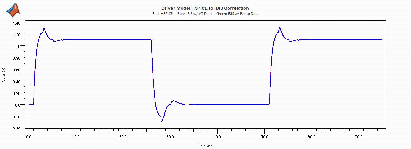
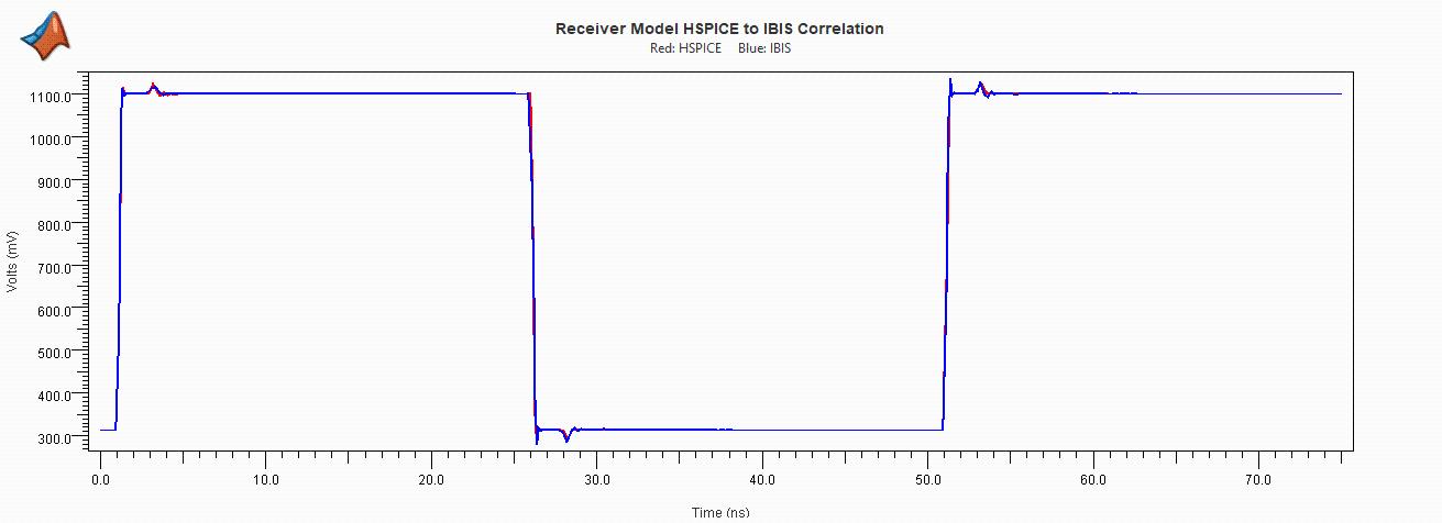
The SPICE (red) and IBIS-VT (blue) waveforms overlap closely, especially during the mid-swing transition and settling regions.
Expect minor differences in the first few picoseconds of the edge launch. IBIS uses a simplified launch model.
The IBIS-Ramp (green) typically shows larger deviations, especially in the settling region and overshoot peaks. This is expected and demonstrates why VT waveform data improves accuracy.
Example driver correlation plots:
Example receiver correlation plots:
Common Correlation Issues
Timing offset. If the IBIS waveform shifts in time relative to SPICE, check the
[Ramp]offset parameter. IBIS Designer extraction handles this automatically.Overshoot amplitude mismatch. If the IBIS model under-predicts overshoot, your clamp IV curves may not extend far enough beyond the supply rails. Verify that the IV sweep range in your extraction covers at least -Vdd to 2*Vdd.
Steady-state offset. A DC offset in the settled waveform indicates an error in the pullup/pulldown IV curves or the supply voltage configuration in the IBIS deck.
Ramp-only model shows large error but VT is good. This is normal and expected. It confirms that VT waveform data is essential for your application.
When to Investigate Further
Investigate if VT peak error exceeds 10% of Vdd.
Different behavior between rising and falling edges suggests an asymmetric extraction error.
If correlation passes at typ but fails at min/max, check your corner parameter configuration.
Receiver Correlation Interpretation
Receiver correlation is fundamentally different from driver correlation, and the metrics mean something narrower. A driver deck exercises the switching edge shape, which is why it instantiates both a VT and a Ramp instance: the gap between them shows how much the VT waveform data adds. A receiver deck has no switching edge to reproduce: it instantiates a VT instance only (no Ramp instance), and the script reports VT metrics only (the Ramp columns print -).
What receiver correlation actually validates:
ODT (on-die termination) resistance and clamp behavior: how the receiver terminates the incoming wave and how its clamps respond to reflections that swing beyond the rails.
Input capacitance (********
C_comp). A receiver can show 99% FOM here and still have the wrongC_comp, because this transient test is dominated by termination, not by the small pad capacitance, however the reflected behavior of the receiver is still influenced by the correct C_comp value.
To verify C_comp accuracy, use an AC impedance comparison instead (see the AC characterization section of Generate HSPICE Simulation Decks for IBIS Characterization). Treat a high receiver FOM as confirmation of termination and clamp behavior, not as a blanket statement that the receiver model is correct in all respects.
Summary
In this topic, you learned:
Why correlation is a critical step in the IBIS model development process
How to design correlation circuits that stress-test both driver switching and clamp behavior
How to use HSPICE's B-element to simulate an IBIS model in the same environment as the SPICE original
How to read and compare transient waveforms in MATLAB with quantitative error metrics
How to interpret correlation results and diagnose common issues
References
I/O Buffer Accuracy Handbook: Defines the Curve Overlay Metric (FOM) used in this topic.

