bilinear

用于模数滤波器转换的双线性变换方法

全页折叠

语法

[zd,pd,kd] = bilinear(z,p,k,fs)

[numd,dend] = bilinear(num,den,fs)

[Ad,Bd,Cd,Dd] = bilinear(A,B,C,D,fs)

[___] = bilinear(___,fp)

说明

使用此函数将连续时间传递函数转换为等效的离散时间函数。

[zd,pd,kd] = bilinear(z,p,k,fs) 将由 z、p、k 和采样率 fs 指定的零极点形式的 s 域传递函数转换为等效的离散函数。

示例

[numd,dend] = bilinear(num,den,fs) 将由分子 num 和分母 den 指定的 s 域传递函数转换为等效的离散函数。

[Ad,Bd,Cd,Dd] = bilinear(A,B,C,D,fs) 将矩阵 A、B、C 和 D 中的连续时间状态空间系统转换为离散时间系统。

示例

[___] = bilinear(___,fp) 使用参数 fp 作为“匹配”频率来指定预修正。

示例

全部折叠

使用切比雪夫 I 型模拟滤波器的带通 IIR 滤波器设计

打开实时脚本

为具有 6 dB 通带波纹的 10 阶切比雪夫 I 型滤波器设计原型。将原型转换为状态空间形式。

[z,p,k] = cheb1ap(10,6);
[A,B,C,D] = zp2ss(z,p,k);

将原型变换为带通滤波器，使得等效数字滤波器在以速率 $f_{s} = 2 kHz$ 采样时其通带边缘位于 100 Hz 和 500 Hz。对于该变换，指定预修正的频带边缘 $u_{1}$ 和 $u_{2}$ （以弧度/秒为单位）、中心频率 $W_{o} = \sqrt{u_{1} u_{2}}$ 和带宽 $B_{w} = u_{2} - u_{1}$ 。

fs = 2e3;

f1 = 100; u1 = 2*fs*tan(f1*(2*pi/fs)/2);
f2 = 500; u2 = 2*fs*tan(f2*(2*pi/fs)/2);

[At,Bt,Ct,Dt] = lp2bp(A,B,C,D,sqrt(u1*u2),u2-u1);

使用 freqs 计算模拟滤波器的频率响应。绘制幅值响应和预修正的频带边缘。

[b,a] = ss2tf(At,Bt,Ct,Dt);
[h,w] = freqs(b,a,2048);

plot(w,mag2db(abs(h)))
xline([u1 u2],"-",["Lower" "Upper"]+" passband edge", ...
    LabelVerticalAlignment="middle")

ylim([-165 5])
xlabel("Angular frequency (rad/s)")
ylabel("Magnitude (dB)")
grid

Figure contains an axes object. The axes object with xlabel Angular frequency (rad/s), ylabel Magnitude (dB) contains 3 objects of type line, constantline.

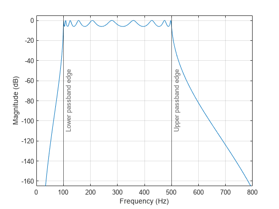
使用 bilinear 函数创建一个采样率为 $f_{s}$ 的数字带通滤波器。

[Ad,Bd,Cd,Dd] = bilinear(At,Bt,Ct,Dt,fs);

将数字滤波器从状态空间形式转换为二阶节，并使用 freqz 计算频率响应。绘制幅值响应和通带边缘。

[hd,fd] = freqz(ss2sos(Ad,Bd,Cd,Dd),2048,fs);

plot(fd,mag2db(abs(hd)))
xline([f1 f2],"-",["Lower" "Upper"]+" passband edge", ...
    LabelVerticalAlignment="middle")

ylim([-165 5])
xlabel("Frequency (Hz)")
ylabel("Magnitude (dB)")
grid

Figure contains an axes object. The axes object with xlabel Frequency (Hz), ylabel Magnitude (dB) contains 3 objects of type line, constantline.

椭圆滤波器的离散时间表示

打开实时脚本

设计一个 6 阶椭圆模拟低通滤波器，其通带波纹为 5 dB，阻带衰减为 90 dB，截止频率为 $f_{c} = 20 Hz$ 。

fc = 20;

[z,p,k] = ellip(6,5,90,2*pi*fc,"s");

可视化模拟椭圆滤波器的幅值响应。显示截止频率。

[num,den] = zp2tf(z,p,k);
[h,w] = freqs(num,den,1024);

plot(w/(2*pi),mag2db(abs(h)))
xline(fc,Color=[0.8500 0.3250 0.0980])

axis([0 100 -125 5])
grid
legend(["Magnitude response" "Cutoff frequency"])
xlabel("Frequency (Hz)")
ylabel("Magnitude (dB)")

Figure contains an axes object. The axes object with xlabel Frequency (Hz), ylabel Magnitude (dB) contains 2 objects of type line, constantline. These objects represent Magnitude response, Cutoff frequency.

使用 bilinear 函数将模拟滤波器变换为离散时间 IIR 滤波器。指定采样率 $f_{s} = 200 Hz$ 和预修正匹配频率 $f_{p} = 20 Hz$ 。

fs = 200;
fp = 20;

[zd,pd,kd] = bilinear(z,p,k,fs,fp);

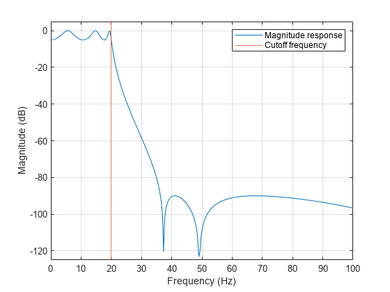
可视化离散时间滤波器的幅值响应。显示截止频率。

[hd,fd] = freqz(zp2sos(zd,pd,kd),[],fs);

plot(fd,mag2db(abs(hd)))
xline(fc,Color=[0.8500 0.3250 0.0980])

axis([0 100 -125 5])
grid
legend(["Magnitude response" "Cutoff frequency"])
xlabel("Frequency (Hz)")
ylabel("Magnitude (dB)")

输入参数

全部折叠

`z`, `p`, `k` — 模拟域零点、极点和增益
列向量、标量

s 域传递函数的零点、极点和增益，指定为两个列向量和一个标量。

`fs` — 采样率
正标量

采样率，指定为正标量。

`num`, `den` — 模拟域分子系数和分母系数
行向量

模拟传递函数的分子系数和分母系数，指定为行向量。

`A`, `B`, `C`, `D` — 模拟域状态空间矩阵
矩阵

s 域中的状态空间表示，指定为矩阵。如果系统有 p 个输入和 q 个输出，并由 n 个状态变量描述，则 A 是 n×n 矩阵，B 是 n×p 矩阵，C 是 q×n 矩阵，D 是 q×p 矩阵。

数据类型: single | double

`fp` — 匹配频率
正标量

匹配频率，指定为正标量。

输出参量

全部折叠

`zd`, `pd`, `kd` — 数字域零点、极点和增益
列向量、标量

z 域传递函数的零点、极点和增益，以列向量和标量形式返回。

`numd`, `dend` — 数字域分子系数和分母系数
行向量

数字传递函数的分子系数和分母系数，以行向量形式返回。

`Ad`, `Bd`, `Cd`, `Dd` — 数字域状态空间矩阵
矩阵

z 域中的状态空间表示，以矩阵形式返回。如果系统由 n 个状态变量描述并有 q 个输出，则 Ad 是 n×n 矩阵，Bd 是 n×1 矩阵，Cd 是 q×n 矩阵，Dd 是 q×1 矩阵。

数据类型: single | double

算法

全部折叠

双线性变换是变量的数学映射。在数字滤波中，它是将 s 或模拟平面映射到 z 或数字平面的标准方法。它将使用经典滤波器设计方法设计的模拟滤波器变换为其等效的离散形式。

双线性变换通过下式将 s 平面映射到 z 平面：

${H (z) = H (s) |}_{s = 2 f_{s} \times \frac{z - 1}{z + 1}} .$

此变换通过下式将 jΩ 轴（从 Ω = –∞ 到 +∞）反复映射到单位圆 e^jω 上（从 ω = –π 到 π）：

$ω = 2 \tan^{- 1} (\frac{Ω}{2 f_{s}}) .$

bilinear 可以接受可选参数 f_p 来指定预修正。f_p（以赫兹为单位）指示匹配频率，映射前后的频率响应在该频率处精确匹配。在预修正模式下，双线性变换通过下式将 s 平面映射到 z 平面：

${H (z) = H (s) |}_{s = \frac{2 π f_{p}}{\tan (π \frac{f_{p}}{f_{s}})} \times \frac{z - 1}{z + 1}} .$

使用预修正选项时，bilinear 通过下式将 jΩ 轴（从 Ω = –∞ 到 +∞）反复映射到单位圆 e^jω 上（从 ω = –π 到 π）：

$ω = 2 \tan^{- 1} (\frac{Ω \tan (π \frac{f_{p}}{f_{s}})}{2 π f_{p}}) .$

在预修正模式下，bilinear 将 s 平面中的频率 2πf_p（以弧度/秒为单位）与 z 平面中的归一化频率 2πf_p/f_s（以弧度/秒为单位）匹配。

bilinear 函数支持三种不同线性系统表示形式：零极点增益、传递函数和状态空间形式。

bilinear 使用两种算法之一，具体使用哪种算法取决于您提供的输入线性系统的形式。一种算法适用于零极点增益形式，另一种算法适用于状态空间形式。对于传递函数表示，bilinear 将其转换为状态空间形式，执行变换，然后将生成的状态空间系统转换回传递函数形式。

零极点增益算法

对于零极点增益形式的系统，bilinear 执行以下四个步骤：

如果存在 fp，则进行预修正：
```
fp = 2*pi*fp;
fs = fp/tan(fp/fs/2)
```
否则，fs = 2*fs。
它使用下式去除位于 ±∞ 处的任何零点：
```
z = z(finite(z));
```

它使用下式变换零点、极点和增益：

pd = (1+p/fs)./(1-p/fs);    % Do bilinear transformation
zd = (1+z/fs)./(1-z/fs);
kd = real(k*prod(fs-z)./prod(fs-p));

它在 -1 处添加额外的零点，以便生成的系统具有相等的分子和分母阶数。

状态空间算法

模拟系统的状态空间方程

$\begin{array}{l} \dot{x} = A x + B u \\ y = C x + D u \end{array}$

可以转换为离散形式：

$\begin{array}{l} x [n + 1] = A_{d} x [n] + B_{d} u [n], \\ y [n] = C_{d} x [n] + D_{d} u [n] . \end{array}$

要进行此转换，bilinear 需要执行两个步骤 [1]：

如果指定了匹配频率 f_p，则让

$λ = \frac{π f_{p}}{\tan (π f_{p} / f_{s})} .$
如果未指定 f_p，则让 λ = f_s。
使用下式计算 A_d、B_d、C_d 和 D_d（用 A、B、C 和 D 表示）：
$\begin{array}{l} A_{d} = (^{I - A \frac{1}{2 λ}) - 1} (I + A \frac{1}{2 λ}), \\ B_{d} = \frac{1}{\sqrt{λ}} (^{I - A \frac{1}{2 λ}) - 1} B, \\ C_{d} = \frac{1}{\sqrt{λ}} C (^{I - A \frac{1}{2 λ}) - 1}, \\ D_{d} = \frac{1}{2 λ} C (^{I - A \frac{1}{2 λ}) - 1} B + D . \end{array}$

传递函数

对于传递函数形式的系统，bilinear 将由 num 和 den 给出的 s 域传递函数转换为等效的离散函数。行向量 num 和 den 分别指定分子和分母的系数，按 s 的降幂顺序。令 B(s) 为分子多项式，A(s) 为分母多项式。传递函数为：

$\frac{B (s)}{A (s)} = \frac{B (1) s^{n} + \dots + B (n) s + B (n + 1)}{A (1) s^{m} + \dots + A (m) s + A (m + 1)}$

fs 是以赫兹为单位的采样率。bilinear 以行向量 numd 和 dend 返回等效的离散函数，按 z 的降幂顺序（即 z^–1 的升幂）。fp 是可选的匹配频率（以赫兹为单位），用于预修正。

参考

[1] Al-Saggaf, Ubaid M., and Gene F. Franklin. “Model Reduction via Balanced Realizations: An Extension and Frequency Weighting Techniques.” IEEE Transactions on Automatic Control 33, no. 7 (July 1988): 687–92. https://doi.org/10.1109/9.1280.

[2] Oppenheim, Alan V., and Ronald W. Schafer, with John R. Buck. Discrete-Time Signal Processing. Upper Saddle River, NJ: Prentice Hall, 1999.

[3] Parks, Thomas W., and C. Sidney Burrus. Digital Filter Design. New York: John Wiley & Sons, 1987.

[4] Tustin, Arnold. “A Method of Analysing the Behaviour of Linear Systems in Terms of Time Series.” Journal of the Institution of Electrical Engineers - Part IIA: Automatic Regulators and Servo Mechanisms 94, no. 1 (May 1947): 130–42. https://doi.org/10.1049/ji-2a.1947.0020.

扩展功能

全部展开

C/C++ 代码生成
使用 MATLAB® Coder™ 生成 C 代码和 C++ 代码。

GPU 代码生成
使用 GPU Coder™ 为 NVIDIA® GPU 生成 CUDA® 代码。

版本历史记录

在 R2006a 之前推出

另请参阅

impinvar | lp2bp | lp2bs | lp2hp | lp2lp

主题

连续-离散转换方法 (Control System Toolbox)

bilinear

语法

说明

示例

使用切比雪夫 I 型模拟滤波器的带通 IIR 滤波器设计

椭圆滤波器的离散时间表示

输入参数

z, p, k — 模拟域零点、极点和增益 列向量、标量

fs — 采样率 正标量

num, den — 模拟域分子系数和分母系数 行向量

A, B, C, D — 模拟域状态空间矩阵 矩阵

fp — 匹配频率 正标量

输出参量

zd, pd, kd — 数字域零点、极点和增益 列向量、标量

numd, dend — 数字域分子系数和分母系数 行向量

Ad, Bd, Cd, Dd — 数字域状态空间矩阵 矩阵

算法

零极点增益算法

状态空间算法

传递函数

参考

扩展功能

C/C++ 代码生成 使用 MATLAB® Coder™ 生成 C 代码和 C++ 代码。

GPU 代码生成 使用 GPU Coder™ 为 NVIDIA® GPU 生成 CUDA® 代码。

版本历史记录

另请参阅

主题

`z`, `p`, `k` — 模拟域零点、极点和增益
列向量、标量

`fs` — 采样率
正标量

`num`, `den` — 模拟域分子系数和分母系数
行向量

`A`, `B`, `C`, `D` — 模拟域状态空间矩阵
矩阵

`fp` — 匹配频率
正标量

`zd`, `pd`, `kd` — 数字域零点、极点和增益
列向量、标量

`numd`, `dend` — 数字域分子系数和分母系数
行向量

`Ad`, `Bd`, `Cd`, `Dd` — 数字域状态空间矩阵
矩阵

C/C++ 代码生成
使用 MATLAB® Coder™ 生成 C 代码和 C++ 代码。

GPU 代码生成
使用 GPU Coder™ 为 NVIDIA® GPU 生成 CUDA® 代码。