chirp
Swept-frequency cosine
Syntax
Description
Examples
Linear Chirp
Generate a chirp with linear instantaneous frequency deviation. The chirp is sampled at 1 kHz for 2 seconds. The instantaneous frequency is 0 at t = 0 and crosses 250 Hz at t = 1 second.
t = 0:1/1e3:2;
y = chirp(t,0,1,250);
Compute and plot the spectrogram of the chirp. Divide the signal into segments such that the time resolution is 0.1 second. Specify 99% of overlap between adjoining segments and a spectral leakage of 0.85.
pspectrum(y,1e3,"spectrogram",TimeResolution=0.1, ...
    OverlapPercent=99,Leakage=0.85)

Quadratic Chirp
Generate a chirp with quadratic instantaneous frequency deviation. The chirp is sampled at 1 kHz for 2 seconds. The instantaneous frequency is 100 Hz at t = 0 and crosses 200 Hz at t = 1 second.
t = 0:1/1e3:2;
y = chirp(t,100,1,200,"quadratic");
Compute and plot the spectrogram of the chirp. Divide the signal into segments such that the time resolution is 0.1 second. Specify 99% of overlap between adjoining segments and a spectral leakage of 0.85.
pspectrum(y,1e3,"spectrogram",TimeResolution=0.1, ...
    OverlapPercent=99,Leakage=0.85)

Convex Quadratic Chirp
Generate a convex quadratic chirp sampled at 1 kHz for 2 seconds. The instantaneous frequency is 400 Hz at t = 0 and crosses 300 Hz at t = 1 second.
t = 0:1/1e3:2;
fo = 400;
f1 = 300;
y = chirp(t,fo,1,f1,"quadratic",[],"convex");
Compute and plot the spectrogram of the chirp. Divide the signal into segments such that the time resolution is 0.1 second. Specify 99% of overlap between adjoining segments and a spectral leakage of 0.85.
pspectrum(y,1e3,"spectrogram",TimeResolution=0.1, ...
    OverlapPercent=99,Leakage=0.85)

Symmetric Concave Quadratic Chirp
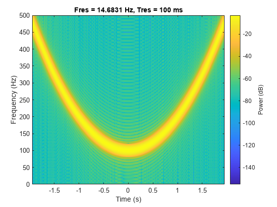
Generate a concave quadratic chirp sampled at 1 kHz for 4 seconds. Specify the time vector so that the instantaneous frequency is symmetric about the halfway point of the sampling interval, with a minimum frequency of 100 Hz and a maximum frequency of 500 Hz.
t = -2:1/1e3:2;
fo = 100;
t1 = max(t);
f1 = 500;
y = chirp(t,fo,t1,f1,"quadratic",[],"concave");
Compute and plot the spectrogram of the chirp. Divide the signal into segments such that the time resolution is 0.1 second. Specify 99% of overlap between adjoining segments and a spectral leakage of 0.85.
pspectrum(y,t,"spectrogram",TimeResolution=0.1, ...
    OverlapPercent=99,Leakage=0.85)

Logarithmic Chirp
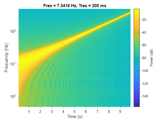
Generate a logarithmic chirp sampled at 1 kHz for 10 seconds. The instantaneous frequency is 10 Hz initially and 400 Hz at the end.
t = 0:1/1e3:10;
fo = 10;
f1 = 400;
y = chirp(t,fo,10,f1,"logarithmic");
Compute and plot the spectrogram of the chirp. Divide the signal into segments such that the time resolution is 0.2 second. Specify 99% of overlap between adjoining segments and a spectral leakage of 0.85.
pspectrum(y,t,"spectrogram",TimeResolution=0.2, ...
    OverlapPercent=99,Leakage=0.85)

Use a logarithmic scale for the frequency axis. The spectrogram becomes a line, with high uncertainty at low frequencies.
ax = gca;
ax.YScale = "log";
Complex Chirp
Generate a complex linear chirp sampled at 1 kHz for 10 seconds using single support precision. The instantaneous frequency is –200 Hz initially and 300 Hz at the end. The initial phase is zero.
fs = 1e3;
t = single(0:1/fs:10);
fo = -200;
f1 = 300;
ph0 = 0;

y = chirp(t,fo,t(end),f1,"linear",ph0,"complex");
Compute and plot the spectrogram of the chirp. Divide the signal into segments such that the time resolution is 0.2 second. Specify 99% of overlap between adjoining segments and a spectral leakage of 0.85.
pspectrum(y,t,"spectrogram",TimeResolution=0.2, ...
    OverlapPercent=99,Leakage=0.85)

Verify that a complex chirp has real and imaginary parts that are equal but with phase difference.
x = chirp(t,fo,t(end),f1,"linear",0)...
    + 1j*chirp(t,fo,t(end),f1,"linear",-90);

pspectrum(x,t,"spectrogram",TimeResolution=0.2, ...
    OverlapPercent=99,Leakage=0.85)

Input Arguments
t — Time array
vector | matrix | N-D array
Time array, specified as a vector, matrix, or N-D array.
If you specify t using single-precision data, the
chirp function generates a single-precision
signal y.
Data Types: single | double
f0 — Instantaneous frequency at time 0
0 (default) | real scalar in Hz
Initial instantaneous frequency at time 0, specified as a real scalar expressed in Hz.
Data Types: single | double
t1 — Reference time
1 (default) | positive scalar in seconds
Reference time, specified as a positive scalar expressed in seconds.
Data Types: single | double
f1 — Instantaneous frequency at time t1
100 (default) | real scalar in Hz
Instantaneous frequency at time t1, specified as a
real scalar expressed in Hz.
Data Types: single | double
method — Sweep method
"linear" (default) | "quadratic" | "logarithmic"
Sweep method, specified as "linear",
"quadratic", or "logarithmic".
"linear"— Specifies an instantaneous frequency sweep fi(t) given bywhere
and the default value for f0 is 0. The coefficient β ensures that the desired frequency breakpoint f1 at time t1 is maintained.
"quadratic"— Specifies an instantaneous frequency sweep fi(t) given bywhere
and the default value for f0 is 0. If f0 > f1 (downsweep), the default shape is convex. If f0 < f1 (upsweep), the default shape is concave.
"logarithmic"— Specifies an instantaneous frequency sweep fi(t) given bywhere
and the default value for f0 is 10–6.
Data Types: char | string
phi — Initial phase
0 (default) | positive scalar in degrees
Initial phase, specified as a positive scalar expressed in degrees.
Data Types: single | double
shape — Spectrogram shape of quadratic chirp
"convex" | "concave"
Spectrogram shape of quadratic chirp, specified as
"convex" or "concave".
shape describes the shape of the parabola with
respect to the positive frequency axis. If not specified,
shape is "convex" for the
downsweep case with f0 >
f1, and
"concave" for the upsweep case with
f0 <
f1.

Data Types: char | string
cplx — Output complexity
"real" (default) | "complex"
Output complexity, specified as "real" or
"complex".
Data Types: char | string
Output Arguments
y — Swept-frequency cosine signal
vector
Swept-frequency cosine signal, returned as a vector.
Extended Capabilities
C/C++ Code Generation
Generate C and C++ code using MATLAB® Coder™.
Thread-Based Environment
Run code in the background using MATLAB® backgroundPool or accelerate code with Parallel Computing Toolbox™ ThreadPool.
This function fully supports thread-based environments. For more information, see Run MATLAB Functions in Thread-Based Environment.
Version History
Introduced before R2006aR2024b: Generate Single-Precision Outputs
The chirp function supports single-precision
outputs.
MATLAB Command
You clicked a link that corresponds to this MATLAB command:
Run the command by entering it in the MATLAB Command Window. Web browsers do not support MATLAB commands.

Select a Web Site
Choose a web site to get translated content where available and see local events and offers. Based on your location, we recommend that you select: .
You can also select a web site from the following list
How to Get Best Site Performance
Select the China site (in Chinese or English) for best site performance. Other MathWorks country sites are not optimized for visits from your location.
Americas
- América Latina (Español)
- Canada (English)
- United States (English)
Europe
- Belgium (English)
- Denmark (English)
- Deutschland (Deutsch)
- España (Español)
- Finland (English)
- France (Français)
- Ireland (English)
- Italia (Italiano)
- Luxembourg (English)
- Netherlands (English)
- Norway (English)
- Österreich (Deutsch)
- Portugal (English)
- Sweden (English)
- Switzerland
- United Kingdom (English)
Asia Pacific
- Australia (English)
- India (English)
- New Zealand (English)
- 中国
- 日本Japanese (日本語)
- 한국Korean (한국어)