Main Content

dutycycle

Duty cycle of pulse waveform

Description

d = dutycycle(x) returns the ratio of pulse width to pulse period for each positive-polarity pulse. The function identifies all regions that cross the upper-state boundary of the low state and the lower-state boundary of the high state. To determine the transitions that define each pulse, dutycycle estimates the state levels of x by a histogram method. The low-state and high-state boundaries are expressed as the state level plus or minus a scalar multiple of the difference between the state levels. See State-Level Tolerances for more details.

example

d = dutycycle(x,fs) specifies the sample rate at which x is sampled. The first sample instant of x corresponds to t = 0.

example

d = dutycycle(x,t) specifies the instants, t, at which x is sampled.

example

[d,initcross,finalcross,nextcross,midlev] = dutycycle(___) with any input arguments from previous syntaxes also returns:

  • A vector, initcross, whose elements correspond to the mid-crossings (mid-reference level instants) of the initial transition of each pulse with a corresponding nextcross.

  • A vector, finalcross, whose elements correspond to the mid-crossings (mid-reference level instants) of the final transition of each pulse with a corresponding nextcross.

  • A vector, nextcross, whose elements correspond to the mid-crossings (mid-reference level instants) of the next detected transition for each pulse.

  • A scalar, midlev, that corresponds to the mid-reference level.

example

[___] = dutycycle(___,Name,Value) returns the ratio of pulse width to pulse period with additional options specified by one or more Name,Value pair arguments.

dutycycle(___) plots the waveform, the location of the mid-reference level instants, the associated reference levels, the state levels, and the associated lower and upper state boundaries.

d = dutycycle(tau,prf) returns the ratio of pulse width to pulse period for a pulse width of tau seconds and a pulse repetition frequency of prf.

Examples

collapse all

Determine the duty cycle of a bilevel waveform. Use the vector indices as the sample instants.

load('pulseex.mat','x')

d = dutycycle(x)
d = 
0.3001

Annotate the result on a plot of the waveform.

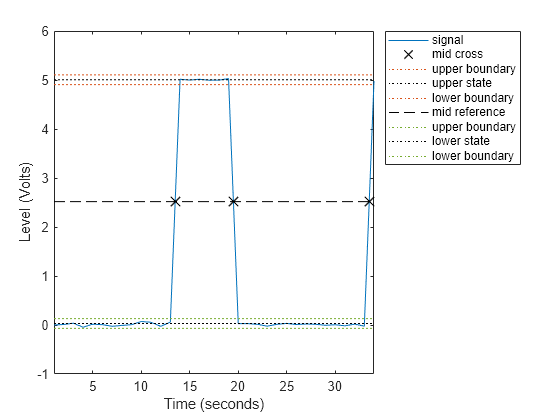
dutycycle(x);

Figure Duty Cycle Plot contains an axes object. The axes object with xlabel Time (seconds), ylabel Level (Volts) contains 9 objects of type line. One or more of the lines displays its values using only markers These objects represent signal, mid cross, upper boundary, upper state, lower boundary, mid reference, lower state.

Determine the duty cycle of a bilevel waveform. The sample rate is 4 MHz.

load('pulseex.mat','x','t')
fs = 1/(t(2)-t(1));

d = dutycycle(x,fs)
d = 
0.3001

Annotate the result on a plot of the waveform.

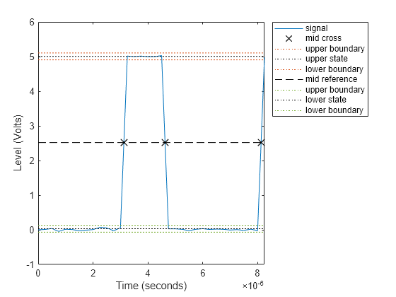
dutycycle(x,fs);

Figure Duty Cycle Plot contains an axes object. The axes object with xlabel Time (seconds), ylabel Level (Volts) contains 9 objects of type line. One or more of the lines displays its values using only markers These objects represent signal, mid cross, upper boundary, upper state, lower boundary, mid reference, lower state.

Create a pulse waveform with three pulses. The sample rate is 4 MHz. Determine the initial and final mid-reference level instants. Plot the result.

load('pulseex.mat','x')
fs = 4e6;

pulse = x(1:30);
wavef = [pulse;pulse;pulse];
t = (0:length(wavef)-1)/fs;

[~,initcross,finalcross,~,midlev] = dutycycle(wavef,t)
initcross = 2×1
10-4 ×

    0.0312
    0.1062

finalcross = 2×1
10-4 ×

    0.0463
    0.1213

midlev = 
2.5177

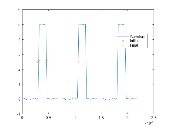
Even though there are three pulses, only two pulses have corresponding subsequent transitions. Plot the result.

plot(t,wavef)
hold on
plot([initcross finalcross],midlev*ones(2),'x','MarkerSize',10)
hold off
legend('Waveform','Initial','Final','Location','best')

Figure contains an axes object. The axes object contains 3 objects of type line. One or more of the lines displays its values using only markers These objects represent Waveform, Initial, Final.

Input Arguments

collapse all

Bilevel waveform, specified as a real-valued vector.

Example: pulstran(0:0.1:10,1:2:9,@rectpuls) specifies a bilevel waveform containing five one-second pulses.

Data Types: double

Sample rate, specified as a positive scalar expressed in Hz.

Data Types: double

Sample instants, specified as a vector of the same length as x.

Data Types: double

Pulse width and repetition frequency, specified as scalars. Express the pulse width in seconds and the repetition frequency in pulses per second. The product of tau and prf must be less than or equal to one.

Data Types: double

Name-Value Arguments

Specify optional pairs of arguments as Name1=Value1,...,NameN=ValueN, where Name is the argument name and Value is the corresponding value. Name-value arguments must appear after other arguments, but the order of the pairs does not matter.

Before R2021a, use commas to separate each name and value, and enclose Name in quotes.

Example: 'MidPercentReferenceLevel',90,'Tolerance',0.5 specifies that the mid-reference level is 90% of the waveform amplitude and the tolerance around the lower- and upper-state boundaries is 0.5%.

Mid-reference level, specified as the comma-separated pair consisting of 'MidPercentReferenceLevel' and a positive scalar expressed as a percentage of the waveform amplitude.

Data Types: double

Pulse polarity, specified as the comma-separated pair consisting of 'Polarity' and either 'positive' or 'negative'.

  • If you specify 'positive', dutycycle looks for pulses with positive-going (positive polarity) initial transitions.

  • If you specify 'negative', dutycycle looks for pulses with negative-going (negative polarity) initial transitions.

See Pulse Polarity for examples of positive and negative-polarity pulses.

Data Types: char

Low- and high-state levels, specified as the comma-separated pair consisting of 'StateLevels' and a 1-by-2 real-valued vector. The first element is the low-state level. The second element is the high-state level. If you do not specify low- and high-state levels, dutycycle estimates the state levels from the input waveform using a histogram method.

Data Types: double

Tolerance levels (lower- and upper-state boundaries), specified as the comma-separated pair consisting of 'Tolerance' and a positive scalar expressed as a percentage. See State-Level Tolerances for more information.

Data Types: double

Output Arguments

collapse all

Duty cycle, returned as a vector or scalar. The elements of d correspond to the ratio of pulse width to pulse period for each pulse in x. d obeys 0 ≤ d ≤ 1 because the pulse width cannot exceed the pulse period. d has length equal to the number of pulse periods in x. If you specify tau and prf as arguments, d is a scalar.

Mid-reference level instants of initial transitions, returned as a vector. The elements of initcross correspond to the mid-crossings (mid-reference level instants) of the initial transition of each pulse with a corresponding nextcross.

Mid-reference level instants of final transitions, returned as a vector. The elements of finalcross correspond to the mid-crossings (mid-reference level instants) of the final transition of each pulse with a corresponding nextcross.

Next transition mid-crossing, returned as a vector. The elements of nextcross correspond to the mid-crossings (mid-reference level instants) of the next detected transition for each pulse.

Mid-reference level waveform value, returned as a scalar. midlevel is a scalar because in a bilevel pulse waveform the state levels are constant.

More About

collapse all

Duty Cycle

The duty cycle of a bilevel pulse is the ratio of average power to peak power.

The energy in a bilevel, or rectangular, pulse is equal to the product of the peak power, Pt, and the pulse width, τ. Devices to measure energy in a waveform operate on time scales longer than the duration of a single pulse. Therefore, it is common to measure the average power

Pav=PtτT,

where T is the pulse period.

The ratio of average power to peak power is the duty cycle:

D=Ptτ/TPt

Pulse Polarity

The polarity of a pulse is defined by the direction of its initial transition.

If the pulse has a positive-going initial transition, the pulse has positive polarity. This figure shows a positive polarity pulse:

Equivalently, a positive-polarity (positive-going) pulse has a terminating state more positive than the originating state.

If the pulse has a negative-going initial transition, the pulse has negative polarity. This figure shows a negative-polarity pulse:

Equivalently, a negative-polarity (negative-going) pulse has an originating state more positive than the terminating state.

State-Level Tolerances

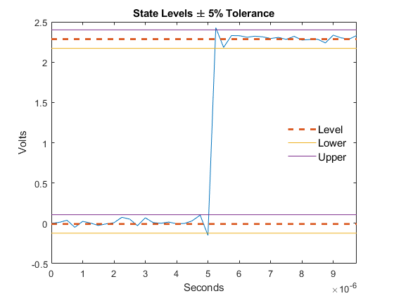
You can specify lower- and upper-state boundaries for each state level. Define the boundaries as the state level plus or minus a scalar multiple of the difference between the high state and the low state. To provide a useful tolerance region, specify the scalar as a small number such as 2/100 or 3/100. In general, the α% region for the low state is defined as

S1±α100(S2-S1),

where S1 is the low-state level and S2 is the high-state level. Replace the first term in the equation with S2 to obtain the α% tolerance region for the high state.

This figure shows lower and upper 5% state boundaries (tolerance regions) for a positive-polarity bi-level waveform. The thick dashed lines indicate the estimated state levels.

0000.png

References

[1] Skolnik, M. I. Introduction to Radar Systems. New York, NY: McGraw-Hill, 1980.

[2] IEEE® Standard on Transitions, Pulses, and Related Waveforms. IEEE Standard 181, 2003.

Extended Capabilities

Version History

Introduced in R2012a