Main Content

lpc

Linear prediction filter coefficients

Description

[a,g] = lpc(x,p) finds the coefficients of a pth-order linear predictor, an FIR filter that predicts the current value of the real-valued time series x based on past samples. The function also returns g, the variance of the prediction error. If x is a matrix, the function treats each column as an independent channel.

example

Examples

collapse all

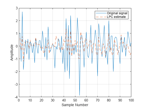
Estimate a data series using a third-order forward predictor. Compare the estimate to the original signal.

First, create the signal data as the output of an autoregressive (AR) process driven by normalized white Gaussian noise. Use the last 4096 samples of the AR process output to avoid startup transients.

noise = randn(50000,1);
x = filter(1,[1 1/2 1/3 1/4],noise);
x = x(end-4096+1:end);

Compute the predictor coefficients and the estimated signal.

a = lpc(x,3);
est_x = filter([0 -a(2:end)],1,x);

Compare the predicted signal to the original signal by plotting the last 100 samples of each.

plot(1:100,x(end-100+1:end),1:100,est_x(end-100+1:end),'--')
grid
xlabel('Sample Number')
ylabel('Amplitude')
legend('Original signal','LPC estimate')

Figure contains an axes object. The axes object with xlabel Sample Number, ylabel Amplitude contains 2 objects of type line. These objects represent Original signal, LPC estimate.

Compute the prediction error and the autocorrelation sequence of the prediction error. Plot the autocorrelation. The prediction error is approximately white Gaussian noise, as expected for a third-order AR input process.

e = x-est_x;
[acs,lags] = xcorr(e,'coeff');

plot(lags,acs)
grid
xlabel('Lags')
ylabel('Normalized Autocorrelation')
ylim([-0.1 1.1])

Figure contains an axes object. The axes object with xlabel Lags, ylabel Normalized Autocorrelation contains an object of type line.

Input Arguments

collapse all

Input array, specified as a vector or matrix. If x is a matrix, then the function treats each column as an independent channel.

Prediction filter polynomial order, specified as a positive integer. p must be less than or equal to the length of x.

Output Arguments

collapse all

Linear predictor coefficients, returned as a row vector or a matrix. The coefficients relate the past p samples of x to the current value:

x^(n)=a(2)x(n1)a(3)x(n2)a(p+1)x(np).

Prediction error variance, returned as a scalar or vector.

More About

collapse all

Prediction Error

The prediction error, e(n), can be viewed as the output of the prediction error filter A(z), where

  • H(z) is the optimal linear predictor.

  • x(n) is the input signal.

  • x^(n) is the predicted signal.

Algorithms

lpc determines the coefficients of a forward linear predictor by minimizing the prediction error in the least squares sense. It has applications in filter design and speech coding.

lpc uses the autocorrelation method of autoregressive (AR) modeling to find the filter coefficients. The generated filter might not model the process exactly, even if the data sequence is truly an AR process of the correct order, because the autocorrelation method implicitly windows the data. In other words, the method assumes that signal samples beyond the length of x are 0.

lpc computes the least-squares solution to Xa = b, where

X=[x(1)00x(2)x(1)x(2)0x(m)x(1)0x(m)x(2)00x(m)],a=[1a(2)a(p+1)],b=[100],

and m is the length of x. Solving the least-squares problem using the normal equations XHXa=XHb leads to the Yule-Walker equations

[r(1)r(2)r(p1)r(p)r(2)r(1)r(p2)r(p1)r(p1)r(p2)r(1)r(2)r(p)r(p1)r(2)r(1)][a(2)a(3)a(p)a(p+1)]=[r(2)r(3)r(p)r(p+1)],

where r = [r(1) r(2) ... r(p+1)] is an autocorrelation estimate for x computed using xcorr. The Levinson-Durbin algorithm (see levinson) solves the Yule-Walker equations in O(p2) flops.

References

[1] Jackson, L. B. Digital Filters and Signal Processing. 2nd Edition. Boston: Kluwer Academic Publishers, 1989, pp. 255–257.
Extended Capabilities

C/C++ Code Generation
Generate C and C++ code using MATLAB® Coder™.

Version History

Introduced before R2006a

expand all