Main Content

undershoot

Undershoot metrics of bilevel waveform transitions

Description

example

us = undershoot(x) returns undershoot expressed as a percentage of the difference between the state levels in the input bilevel waveform. The values in us correspond to the greatest deviations below the final state levels of each transition.

us = undershoot(x,fs) specifies the sample rate fs in hertz.

example

us = undershoot(x,t) specifies the sample instants t.

example

[us,uslev,usinst] = undershoot(___) returns the levels uslev and sample instants usinst of the undershoots for each transition. Specify an input combination from any of the previous syntaxes.

example

[___] = undershoot(___,Name,Value) specifies additional options using one or more name-value arguments.

example

undershoot(___) plots the bilevel waveform and marks the location of the undershoot of each transition. The function also plots the lower and upper reference-level instants and associated reference levels and the state levels and associated lower- and upper-state boundaries.

Examples

collapse all

Determine the maximum percent undershoot relative to the high-state level in a 2.3 V clock waveform.

Load the 2.3 V clock data. Determine the maximum percent undershoot of the transition. Determine also the level and sample instant of the undershoot. In this example, the maximum undershoot in the posttransition region occurs near index 23.

load('transitionex.mat','x')

[uu,lv,nst] = undershoot(x)
uu = 4.5012
lv = 2.1826
nst = 23

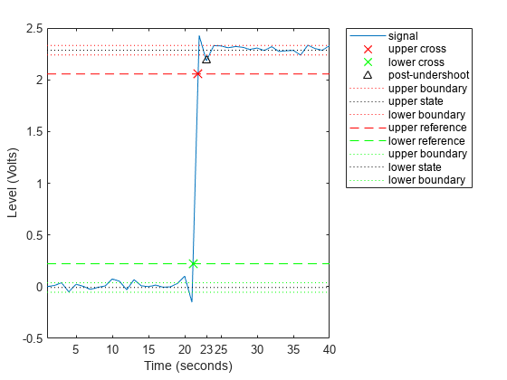
Plot the waveform. Annotate the overshoot and the corresponding sample instant.

undershoot(x);

ax = gca;
ax.XTick = sort([ax.XTick nst]);

Determine the maximum percent undershoot relative to the high-state level, the level of the undershoot, and the sample instant in a 2.3 V clock waveform.

Load the 2.3 V clock data with sampling instants. The clock data are sampled at 4 MHz.

load('transitionex.mat','x','t')

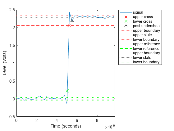
Determine the maximum percent undershoot, the level of the undershoot in volts, and the time instant where the maximum undershoot occurs. Plot the result.

[us,uslev,usinst] = undershoot(x,t)
us = 4.5012
uslev = 2.1826
usinst = 5.5000e-06
undershoot(x,t);

Determine the maximum percent undershoot relative to the low-state level, the level of the undershoot, and the sample instant in a 2.3 V clock waveform. Specify the 'Region' as 'Preshoot' to output pretransition metrics.

Load the 2.3 V clock data with sampling instants. The clock data are sampled at 4 MHz.

load('transitionex.mat','x','t')

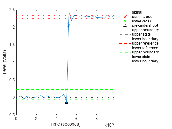
Determine the maximum percent undershoot, the level of the undershoot in volts, and the sampling instant where the maximum undershoot occurs. Plot the result.

[us,uslev,usinst] = undershoot(x,t,'Region','Preshoot')
us = 6.1798
uslev = -0.1500
usinst = 5.0000e-06
undershoot(x,t,'Region','Preshoot');

Input Arguments

collapse all

Bilevel waveform, specified as a real-valued row or column vector. The sample instants in X correspond to the vector indices. The first sample instant in x corresponds to t = 0.

Sample rate in hertz, specified as a real positive scalar. The sample rate determines the sample instants corresponding to the elements in x.

Sample instants, specified as a vector. The length of t must equal the length of the input bilevel waveform x.

Name-Value Arguments

Specify optional pairs of arguments as Name1=Value1,...,NameN=ValueN, where Name is the argument name and Value is the corresponding value. Name-value arguments must appear after other arguments, but the order of the pairs does not matter.

Before R2021a, use commas to separate each name and value, and enclose Name in quotes.

Example: 'Tolerance',5 computes the undershoot with a 5% tolerance region.

Reference levels as a percentage of the waveform amplitude, specified as a 1-by-2 real-valued vector. The function defines the lower-state level to be 0 percent and the upper-state level to be 100 percent. The first element corresponds to the lower percent reference level and the second element corresponds to the upper percent reference level.

Aberration region over which to compute the undershoot, specified as 'Preshoot' or 'Postshoot'. If you specify 'Preshoot', the function defines the end of the pretransition aberration region as the last instant when the signal exits the first state. If you specify 'Postshoot', the function defines the start of the posttransition aberration region as the instant when the signal enters the second state. By default, the function computes undershoots for posttransition aberration regions.

Aberration region duration, specified as a real-valued scalar. The function computes the undershoot over the specified duration for each transition as a multiple of the corresponding transition duration. If the edge of the waveform is reached or a complete intervening transition is detected before the aberration region duration elapses, the duration is truncated to the edge of the waveform or the start of the intervening transition.

Low- and high-state levels, specified as a 1-by-2 real-valued vector. The first element corresponds to the low-state level and the second element corresponds to the high-state level of the input waveform.

Tolerance level, specified as a real-valued scalar. The function expresses tolerance as a percentage of the difference between the upper- and lower-state levels. The initial and final levels of each transition must be within the respective state levels.

Output Arguments

collapse all

Undershoots expressed as a percentage of the state levels, returned as a vector. The length of us corresponds to the number of transitions detected in the input signal. For more information, see Undershoot.

Undershoot level, returned as a column vector.

Sample instants of pretransition or posttransition undershoots, returned as a column vector. If you specify fs or t, the undershoot instants are in seconds. If you do not specifyfs or t, the undershoot instants are the indices of the input vector.

More About

collapse all

State-Level Estimation

To determine the transitions, the undershoot function estimates the state levels of the input bilevel waveform x by a histogram method with these steps.

  1. Determine the minimum and maximum amplitudes of the data.

  2. For the specified number of histogram bins, determine the bin width, which is the ratio of the amplitude range to the number of bins.

  3. Sort the data values into the histogram bins.

  4. Identify the lowest and highest indexed histogram bins with nonzero counts.

  5. Divide the histogram into two subhistograms.

  6. Compute the state levels by determining the mode or mean of the upper and lower histograms.

The function identifies all regions that cross the upper-state boundary of the low state and the lower-state boundary of the high state. The low-state and high-state boundaries are expressed as the state level plus or minus a multiple of the difference between the state levels.

Undershoot

The function computes the undershoot percentages based on the greatest deviation from the final state level in each transition.

For a positive-going (positive-polarity) pulse, the undershoot is given by

100(S2U)(S2S1)

where U is the greatest deviation below the high-state level, S2 is the high state, and S1 is the low state.

For a negative-going (negative-polarity) pulse, the undershoot is given by

100(S1U)(S2S1)

This figure shows the calculation of undershoot for a positive-going transition.

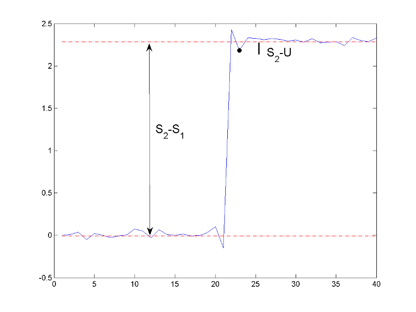
The red dashed lines indicate the estimated state levels. The double-sided black arrow depicts the difference between the high- and low-state levels. The solid black line indicates the difference between the high-state level and the undershoot value.

State-Level Tolerances

You can specify lower- and upper-state boundaries for each state level. Define the boundaries as the state level plus or minus a scalar multiple of the difference between the high state and the low state. To provide a useful tolerance region, specify the scalar as a small number such as 2/100 or 3/100. In general, the $\alpha\%$ region for the low state is defined as

$$S_1\pm{\alpha\over{100}}(S_2-S_1),$$

where $S_1$ is the low-state level and $S_2$ is the high-state level. Replace the first term in the equation with $S_2$ to obtain the $\alpha\%$ tolerance region for the high state.

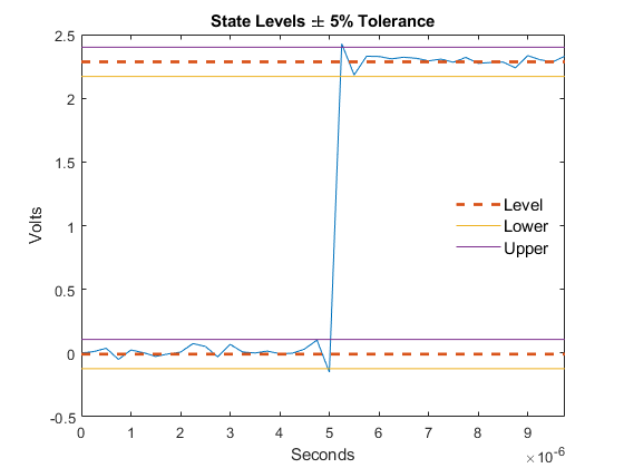
This figure shows lower and upper 5% state boundaries (tolerance regions) for a positive-polarity bilevel waveform. The thick dashed lines indicate the estimated state levels.

References

[1] IEEE Standard 181. IEEE® Standard on Transitions, Pulses, and Related Waveforms (2003): 15–17.

Extended Capabilities

C/C++ Code Generation
Generate C and C++ code using MATLAB® Coder™.

Version History

Introduced in R2012a