Anomaly Detection Using Convolutional Autoencoder with Wavelet Scattering Sequences

Dataset Description and Download

The dataset consists of acoustic recordings collected on a single-stage reciprocating-type air compressor [1]. The data are sampled at 16 kHz. Specifications of the air compressor are as follows:

Each recording represents one of 8 states which includes the healthy state and 7 faulty states. The 7 faulty states are:

In this example the focus is only on normal (healthy) air compressors and those with bearing faults.

Download the dataset and unzip the data file in a folder where you have write permission. This example assumes you are downloading the data in the temporary directory designated as tempdir in MATLAB®. If you choose to use a different folder, substitute that folder for tempdir in the following. The recordings are stored as .wav files in folders named for their respective condition.

url = 'https://www.mathworks.com/supportfiles/audio/AirCompressorDataset/AirCompressorDataset.zip';
downloadFolder = fullfile(tempdir,'AirCompressorDataSet');
if ~exist(fullfile(tempdir,'AirCompressorDataSet'),'dir') 
    loc = websave(downloadFolder,url); 
    unzip(loc,fullfile(tempdir,'AirCompressorDataSet')) 
 end

Because the data are stored in .wav files, use an audioDatastore to manage data access. Each subfolder contains only recordings of the designated class. Use the folder names as the class labels.

rng("default")
ads = audioDatastore(downloadFolder,IncludeSubfolders=true,...
    LabelSource="foldernames"); 

This example focuses only on differentiating recordings obtained in a normally functioning air compressor from those with bearing faults. Create a training set consisting of 50% of the recordings, a validation set consisting of 20%, and a hold-out test set consisting of 30%.

[adsTrain,adsValidation,adsTest] = splitEachLabel(ads,0.5,0.2,0.3,...
    Include=["Healthy","Bearing"]);

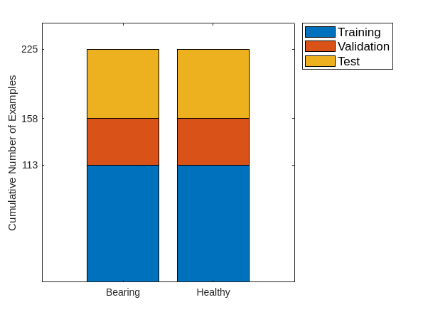
Show the number of examples in each category for the three sets. There are 113 examples in both the normal and faulty categories for the training data, 45 in each class for the validation data, and 67 in each class for the test data. Note that the training and validation data are only necessary for the normal data. Subsequently, the recordings with bearing faults in the training, validation, and test sets will be combined because the anomaly detector does not see those recordings during training and validation.

C = categories(adsTrain.Labels);
categoriesToRemove = C(~ismember(C,unique(adsTrain.Labels)));
uniqueLabels = unique(removecats(adsTrain.Labels,categoriesToRemove));
tblTrain = countEachLabel(adsTrain);
tblValidation = countEachLabel(adsValidation);
tblTest = countEachLabel(adsTest);
H = bar(uniqueLabels,[tblTrain.Count, tblValidation.Count, tblTest.Count],'stacked');
ax = gca;
ax.YTick = [113 113+45 113+45+67];
ax.YLabel.String = "Cumulative Number of Examples";
legend(H,["Training","Validation","Test"],Location="NorthEastOutside",FontSize=12)

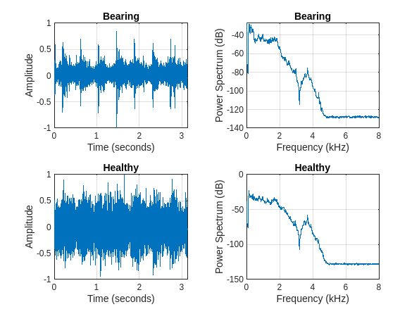
Plot one randomly selected signal and its power spectrum from each class in the training set for illustration purposes.

tiledlayout(2,2)
for n = 1:numel(uniqueLabels)
    idx = find(adsTrain.Labels==uniqueLabels(n),1);
    [x,fs] = audioread(adsTrain.Files{idx});    
    t = (0:size(x,1)-1)/fs;
    nexttile
    plot(t,x);
    grid on
    xlabel("Time (seconds)")
    ylabel("Amplitude")
    title(string(uniqueLabels(n)));
    nexttile
    pspectrum(x,fs)
    title(string(uniqueLabels(n)));
end

Wavelet Scattering Network

Construct the wavelet scattering network. Set the invariance scale to 0.3 seconds for a sample rate of 16 kHz which corresponds to 4800 samples. Set the base-2 logarithm of the oversampling factor to 1 to reduce the amount of downsampling by a factor of 2. These settings result in 98 coefficients per scattering path and 324 paths in total.

N = 5e4;
sn = waveletScattering(SignalLength=N,SamplingFrequency=fs,...
    InvarianceScale=0.3,OversamplingFactor=1); 
numCoefficients(sn)

ans = 98

[~,npaths] = paths(sn);
sum(npaths)

ans = 324

Set up the batch processing for obtaining the wavelet scattering coefficients for the training, validation, and test sets. The processing of the scattering coefficients is done by the helper function, helperbatchscatfeatures, included at the end of this example. Each signal is standardized to have zero mean and unit standard deviation before obtaining the scattering coefficients. Additionally, the data are cast to single precision. In this example, an NVIDIA® Titan V GPU is used to speed up the computation of the scattering coefficients. If you do not access to a GPU with sufficient compute capability, you can set useGPU to false.

useGPU = true; 
batchsize = 64;
scTrain = [];
reset(adsTrain)
while hasdata(adsTrain)
    sc = helperbatchscatfeatures(adsTrain,sn,N,batchsize,useGPU);
    scTrain = cat(3,scTrain,sc);
end

Repeat the same process for the validation and test sets.

scValidation = [];
reset(adsValidation)
while hasdata(adsValidation)
   sc = helperbatchscatfeatures(adsValidation,sn,N,batchsize,useGPU);
   scValidation = cat(3,scValidation,sc); 
end
scTest = [];
reset(adsTest)
while hasdata(adsTest)
   sc = helperbatchscatfeatures(adsTest,sn,N,batchsize,useGPU);
   scTest = cat(3,scTest,sc); 
end

For each of the scattering coefficients remove the 0th order coefficients and put the scattering coefficients in cell arrays for use in the deepSignalAnomalyDetector. This reduces the number of scattering paths (channels) to 323.

trainFeatures = scTrain(2:end,:,:);
trainFeatures = squeeze(num2cell(trainFeatures,[1 2])); 
trainLabels = adsTrain.Labels;
validationFeatures = scValidation(2:end,:,:);
validationFeatures = squeeze(num2cell(validationFeatures,[1 2]));
validationLabels = adsValidation.Labels;
testFeatures = scTest(2:end,:,:);
testFeatures = squeeze(num2cell(testFeatures,[1 2]));
testLabels = adsTest.Labels;

To prepare for training and testing, subset the training, validation, and test sets into the two classes. Note that normal ("Healthy") data is used to train the detector and for validation.

trainNormal = trainFeatures(trainLabels=="Healthy");
trainFaulty = trainFeatures(trainLabels=="Bearing");
validationNormal = validationFeatures(validationLabels=="Healthy");
validationFaulty = validationFeatures(validationLabels=="Bearing");
testNormal = testFeatures(testLabels=="Healthy");
testFaulty = testFeatures(testLabels=="Bearing");
testLabels = removecats(testLabels,categoriesToRemove);

Transpose the scattering coefficients into time-by-channel for input into the deepSignalAnomalyDetector.

trainNormal = cellfun(@transpose,trainNormal,UniformOutput=false);
validationNormal = cellfun(@transpose,validationNormal,UniformOutput=false);
testNormal = cellfun(@transpose,testNormal,UniformOutput=false);
trainFaulty = cellfun(@transpose,trainFaulty,UniformOutput=false);
validationFaulty = cellfun(@transpose,validationFaulty,UniformOutput=false);
testFaulty = cellfun(@transpose,testFaulty,UniformOutput=false);

Combine the faulty training, validation, and test data into one dataset consisting of 225 examples labeled testFaulty.

testFaulty = cat(1,trainFaulty,validationFaulty,testFaulty);

Perform similar preparations for the raw data.

reset(adsTrain)
reset(adsValidation)
reset(adsTest)
trainSequences = readall(adsTrain);
validationSequences = readall(adsValidation);
testSequences = readall(adsTest);

Similar to what was done with the scattering sequences, standardize the time series prior to training and testing. Subset the standardized sequences into the normal and faulty classes.

trainSequences = cellfun(@(x)(x-mean(x))./std(x),trainSequences,UniformOutput=false);
validationSequences = cellfun(@(x)(x-mean(x))./std(x),validationSequences,UniformOutput=false);
testSequences = cellfun(@(x)(x-mean(x))./std(x),testSequences,UniformOutput=false);
normalTrainSequences = trainSequences(adsTrain.Labels == "Healthy");
normalValidationSequences = validationSequences(adsValidation.Labels=="Healthy");
normalTestSequences = testSequences(adsTest.Labels=="Healthy");
faultyTrainSequences = trainSequences(adsTrain.Labels == "Bearing");
faultyValidationSequences = trainSequences(adsValidation.Labels == "Bearing");
faultyTestSequences = testSequences(adsTest.Labels=="Bearing");

Combine the training, validation, and test sets for the faulty data into one set consisting of 225 recordings for model testing.

faultySequences = cat(1,faultyTrainSequences,faultyValidationSequences,faultyTestSequences);

Training

In this section, the deepSignalAnomalyDetector is trained using both the scattering sequences and the raw data. The training options use a suitable GPU if available. For the Titan V GPU used in this example, training requires about four minutes for each model. If you wish to skip the training, set trainModels to false and proceed to the Testing section of the example where you can load the pre-trained anomaly detectors.

Use the default deepSignalAnomalyDetector architecture, which is a convolutional autoencoder. Set the window length to use the entire time window in both cases. First, set up the deep signal anomaly detector for the scattering sequences. Here the number of channels is equal to one less than the number of scattering paths because the 0th order scattering coefficients have been removed.

trainModels = true;
if trainModels
    numChannels = size(trainNormal{1},2);
    dsadSCAT = deepSignalAnomalyDetector(numChannels,WindowLength="fullSignal");
end

Next, set up the anomaly detector for the raw data. Here the number of channels is equal to 1.

if trainModels
    numChannels = 1;
    dsadRAW = deepSignalAnomalyDetector(numChannels,WindowLength="fullSignal");
end

Set up the training options. Use an Adam optimizer, a minibatch size of 16, and shuffle the data each epoch. Run the training for 300 epochs. Because the validation data is different for the scattering sequences and the raw data, you need to define two separate trainingOptions objects. Those objects only differ in the included validation data sets.

if trainModels
    optsSCAT = trainingOptions("adam", MaxEpochs=300,MiniBatchSize=16, ...
        ValidationData={validationNormal,validationNormal},...
        Shuffle="every-epoch",...
        OutputNetwork = "best-validation-loss",...
        Verbose=false,Plots="training-progress"); 
    optsRAW = trainingOptions("adam",MaxEpochs=300,MiniBatchSize=16, ...
        ValidationData={normalValidationSequences,normalValidationSequences},... 
        OutputNetwork = "best-validation-loss",...
        Verbose=false,Plots="training-progress");
end

Train the detector using the scattering sequences.

if trainModels
    trainDetector(dsadSCAT,trainNormal,optsSCAT)
end

Repeat the training for raw data if trainModels is true.

if trainModels
    trainDetector(dsadRAW,normalTrainSequences,optsRAW)
end

Testing

If you elected to skip training by setting trainModels to false, you can load the pre-trained models with the following code.

if ~trainModels
    load dsadSCAT.mat %#ok<*UNRCH>
    load dsadRAW.mat
end

To assess the trained models, start by plotting the reconstruction loss distributions for the normal and faulty recordings. The following does this for the model trained with wavelet scattering sequences.

figure
figh = plotLossDistribution(dsadSCAT,testNormal,testFaulty);
figh.Children(1).String = ["Healthy","Bearing","Normal CDF","Faulty CDF"];
ax = gca;
ax.Title.String = "Reconstruction Loss -- Scattering Sequences";

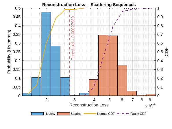
The probability histograms for the reconstruction losses for the normal and faulty classes demonstrate a very good separation. Determine the accuracy of the model on the held-out test set and plot the confusion chart.

First, create a categorical vector consisting of all the test set labels.

fullTestLabels = cat(1,trainLabels(trainLabels=="Bearing"),validationLabels(validationLabels=="Bearing"),testLabels(testLabels=="Bearing"),testLabels(testLabels=="Healthy"));
fullTestLabels = removecats(fullTestLabels,categoriesToRemove);
predNormalSCAT = detect(dsadSCAT,testNormal);
predBearingSCAT = detect(dsadSCAT,testFaulty);
predSCAT = cat(1,cell2mat(predBearingSCAT),cell2mat(predNormalSCAT));
predSCAT = categorical(predSCAT,[1 0],["Bearing" "Healthy"]);
cm = confusionchart(fullTestLabels,predSCAT);
cm.RowSummary = "row-normalized";
cm.ColumnSummary = "column-normalized";
cm.Title = "Wavelet Scattering Sequences with deepSignalAnomalyDetector";

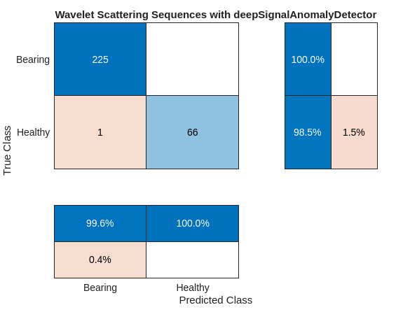
In terms of precision (positive predictive value) and recall (sensitivity), the deepSignalAnomalyDetector paired with the wavelet scattering sequences performs quite well. You can use getModel with the deepSignalAnomalyDetector to see the convolutional architecture the detector trained and uses for detection.

SCATMdl = getModel(dsadSCAT);
SCATMdl.Layers

ans = 
  16×1 Layer array with layers:

     1   'sequenceinput'         Sequence Input               Sequence input with 323 dimensions
     2   'padding'               Function                     @(X)cat(3,X,zeros(size(X,1),size(X,2),ceil(size(X,3)/minLength)*minLength-size(X,3)))
     3   'conv1d_1'              1-D Convolution              32 8×323 convolutions with stride 2 and padding 'same'
     4   'relu_1'                ReLU                         ReLU
     5   'dropout_1'             Dropout                      20% dropout
     6   'conv1d_2'              1-D Convolution              32 8×32 convolutions with stride 2 and padding 'same'
     7   'relu_2'                ReLU                         ReLU
     8   'dropout_2'             Dropout                      20% dropout
     9   'transposed-conv1d_1'   1-D Transposed Convolution   1-D transposed convolution with 32 filters of size 8, stride 2, and cropping 'same'
    10   'relu_3'                ReLU                         ReLU
    11   'dropout_3'             Dropout                      20% dropout
    12   'transposed-conv1d_2'   1-D Transposed Convolution   1-D transposed convolution with 32 filters of size 8, stride 2, and cropping 'same'
    13   'relu_4'                ReLU                         ReLU
    14   'dropout_4'             Dropout                      20% dropout
    15   'fc'                    Fully Connected              323 fully connected layer
    16   'truncating'            Function                     @(X,Y)X(1:size(Y,1),1:size(Y,2),1:size(Y,3))

Plot the reconstruction loss distributions for the anomaly detector trained on the raw time series.

figure
figh = plotLossDistribution(dsadRAW,normalTestSequences,faultySequences);
figh.Children(1).String = ["Normal","Faulty","Normal CDF","Faulty CDF"];
ax = gca;
ax.Title.String = "Reconstruction Loss Distribution -- Raw Data";

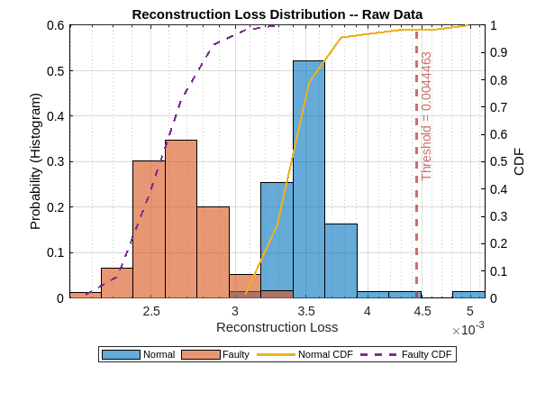
The reconstruction loss distributions for the two classes demonstrate a puzzling reversal in the case of the raw data. Specifically, the reconstruction loss distribution loss for the normal data is shifted to the right of the faulty-data distribution. The overall range of the loss is small indicating that there is not much reconstruction loss for either class. Given the threshold indicated on the plot, you can infer that this model will perform very poorly. In fact, it is likely to simply classify the vast majority of signals as normal.

You can confirm this by running the following code, but in this case you can already discern this information from the plot of the reconstruction loss distributions.

predHealthyRAW = detect(dsadRAW,normalTestSequences);
predBearingRAW = detect(dsadRAW,faultySequences);
predRAW = cat(1,cell2mat(predBearingRAW),cell2mat(predHealthyRAW));
predRAW = categorical(predRAW,[1 0],["Bearing" "Healthy"]);
cm = confusionchart(fullTestLabels,predRAW);
cm.RowSummary = "row-normalized";
cm.ColumnSummary = "column-normalized";
cm.Title = "Raw Sequences with deepSignalAnomalyDetector";

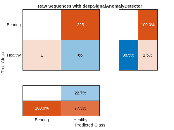
None of the 225 faulty signals has been correctly diagnosed to contain anomalies, while one normal signal has been falsely classified as faulty. One useful diagnostic to assess what has happened in using the deep signal anomaly detector on raw data is to use, plotAnomalies, to plot the anomalies along with the reconstruction loss for sample waveforms from the normal and faulty test sets.

idx = randi(numel(normalTestSequences));
plotAnomalies(dsadRAW,normalTestSequences{idx},PlotReconstruction=true)
title("Normal Sequence With Reconstruction Loss")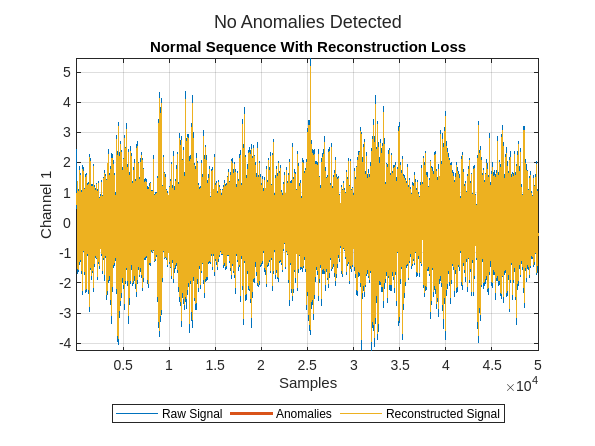

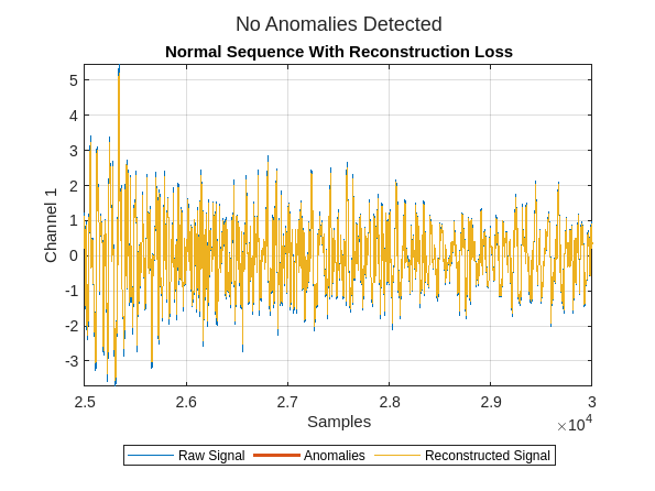
Zoom in on the plot to see the reconstruction in more detail.

xlim([2.5e4 3e4])

Next plot the reconstruction for a randomly selected sequence with a bearing fault. Zoom in to see the reconstruction in more detail.

figure
plotAnomalies(dsadRAW,faultySequences{idx},PlotReconstruction=true)
xlim([2.5e4 3e4])
title("Faulty Sequence With Reconstruction Loss")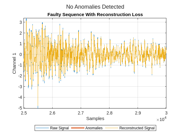

You see the data has been reconstructed almost perfectly (without loss) in both cases. Ideally, the reconstruction loss would be small for the normal data and much larger for the faulty data. It is clear that the anomaly detector has not learned to differentiate normal from faulty signals in this configuration.

Summary

This example has demonstrated the deepSignalAnomalyDetector can perform remarkably better in certain applications if data-centric AI principles are used. In data-centric AI, the focus is often more on the data input to the network rather than the network architecture. Here, the use of wavelet scattering sequences greatly improved the ability of the anomaly detector to differentiate normal from faulty recordings. The key to the success of wavelet scattering in this application is that the scattering transform provides a robust time-frequency feature extractor.

References

[1] N. K. Verma, R. K. Sevakula, S. Dixit and A. Salour, "Intelligent Condition Based Monitoring Using Acoustic Signals for Air Compressors," in IEEE Transactions on Reliability, vol. 65, no. 1, pp. 291-309, March 2016, doi: 10.1109/TR.2015.2459684.

Appendix

Helper functions for the example.

function sc = helperbatchscatfeatures(ds,sn,N,batchsize,useGPU)
% This function is only intended to support examples in the Signal
% Processing and Wavelet Toolboxes. It may be changed or removed in a future
% release.
% Read batch of data from audio datastore
batch = helperReadBatch(ds,N,batchsize);
if useGPU
    batch = gpuArray(batch);
end
% Obtain scattering features. First standardize the batch.
batch = (batch-mean(batch))./std(batch,[],1);
S = sn.featureMatrix(batch);
gather(batch);
S = gather(S);
sc = S;
end

function batchout = helperReadBatch(ds,N,batchsize)
% This function is only intended to support examples in the Signal
% Processing and Wavelet Toolboxes. It may change or be removed in a future
% release.
kk = 1;
while(hasdata(ds)) && kk <= batchsize
    tmpRead = read(ds);
    batchout(:,kk) = cast(tmpRead(1:N),"single"); %#ok<AGROW>
    kk = kk+1;
end
end