Modal Analysis of Identified Models

Hammer Excitation

Load a file containing three-input/three-output hammer excitation data sampled at 4 kHz. Use the first ${10}^4$ samples for estimation and samples $2\times {10}^4$ to $5\times {10}^4$ for model quality validation. Specify the sample time as the inverse of the sample rate. Store the data as @iddata objects.

load modaldata XhammerMISO1 YhammerMISO1 fs

rest = 1:1e4;
rval = 2e4:5e4;
Ts = 1/fs;

Estimation = iddata(YhammerMISO1(rest,:),XhammerMISO1(rest,:),Ts);
Validation = iddata(YhammerMISO1(rval,:), ...
    XhammerMISO1(rval,:),Ts,Tstart=rval(1)*Ts);

Plot the estimation data and the validation data.

plot(Estimation,Validation)
legend(gca,"show")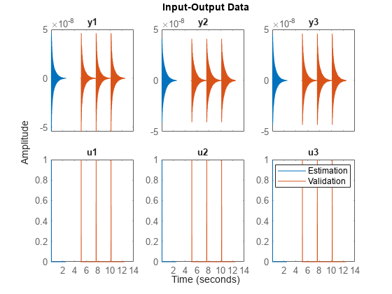

Use the ssest function to estimate a 7th-order state-space model of the system that minimizes the simulation error between the measured outputs and the model outputs. Specify that the state-space model has feedthrough.

Orders = 7;
opt = ssestOptions("Focus","simulation");

sys = ssest(Estimation,Orders,"Feedthrough",true,"Ts",Ts,opt);

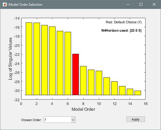
(To find the model order that gives the best tradeoff between accuracy and complexity, set Orders to 1:15 in the previous code. ssest outputs a log plot of singular values that lets you specify the order interactively. The function also recommends a model order of 7.)

Validate the model quality on the validation dataset. Plot the normalized root mean square error (NRMSE) measure of goodness-of-fit. The model describes accurately the output signals of the validation data.

compare(Validation,sys)

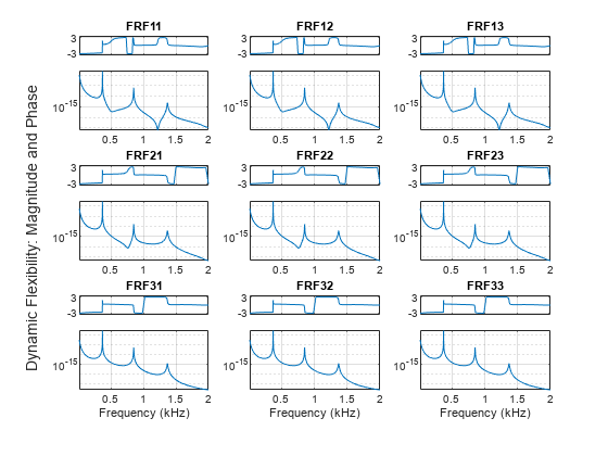
Estimate the frequency-response functions of the model. Display the functions using modalfrf without output arguments.

[frf,f] = modalfrf(sys);
modalfrf(sys)

Assume that the system is well described using three modes. Compute the natural frequencies, damping ratios, and mode-shape vectors of the three modes.

Modes = 3;
[fn,dr,ms] = modalfit(sys,f,Modes)

fn = 3×1
103 ×

    0.3727
    0.8524
    1.3705

dr = 3×1

    0.0008
    0.0013
    0.0030

ms = 3×3 complex

   0.0036 - 0.0019i   0.0036 - 0.0003i   0.0021 + 0.0007i
   0.0043 - 0.0023i   0.0009 - 0.0001i  -0.0034 - 0.0010i
   0.0040 - 0.0021i  -0.0028 + 0.0003i   0.0011 + 0.0003i

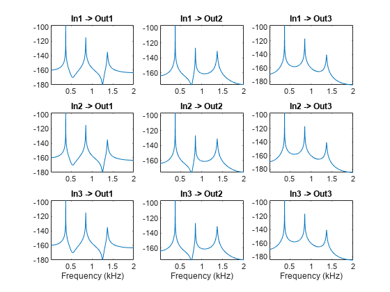
Compute and display the reconstructed frequency-response functions. Express the magnitudes in decibels.

[~,~,~,ofrf] = modalfit(sys,f,Modes);

clf
for ij = 1:3
    for ji = 1:3
        subplot(3,3,3*(ij-1)+ji)
        plot(f/1000,20*log10(abs(ofrf(:,ji,ij))))
        axis tight
        title(sprintf('In%d -> Out%d',ij,ji))
        if ij==3
            xlabel('Frequency (kHz)')
        end
    end
end

Controlled Unstable Process

Load a file containing a high modal density frequency-response measurement. The data corresponds to an unstable process maintained at equilibrium using feedback control. Store the data as an idfrd object for identification. Plot the Bode diagram.

load HighModalDensData FRF f

G = idfrd(permute(FRF,[2 3 1]),f,0,'FrequencyUnit','Hz');
figure
bodemag(G)
xlim([0.01,2e3])

Identify a transfer function with 32 poles and 32 zeros.

sys = tfest(G,32,32);

Compare the frequency response of the model with the measured response.

bodemag(G,sys)
xlim([0.01,2e3])
legend(gca,'show')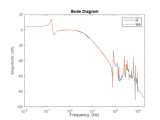

Extract the natural frequencies and damping ratios of the first 10 least-damped oscillatory modes. Store the results in a table.

[fn10,dr10] = modalfit(sys,[],10);
T = table((1:10)',fn10,dr10, ...
    VariableNames=["Mode" "Frequency" "Damping"])

T=10×3 table
    Mode    Frequency     Damping 
    ____    _________    _________

      1      82.764       0.011304
      2      85.013       0.015632
      3      124.04       0.025252
      4      142.04       0.017687
      5      251.46      0.0062182
      6      332.79      0.0058266
      7      401.21      0.0043645
      8      625.14      0.0039247
      9      770.49       0.002795
     10      943.64      0.0019943

Copyright 2017-2024, The MathWorks, Inc.