modalfit

Modal parameters from frequency-response functions

Syntax

fn = modalfit(frf,f,fs,mnum)

fn = modalfit(frf,f,fs,mnum,Name,Value)

[fn,dr,ms]
= modalfit(___)

[fn,dr,ms,ofrf]
= modalfit(___)

[___] = modalfit(sys,f,mnum,Name,Value)

Description

fn = modalfit(frf,f,fs,mnum) estimates the natural frequencies of mnum modes of a system with measured frequency-response functions frf defined at frequencies f and for a sample rate fs. Use modalfrf to generate a matrix of frequency-response functions from measured data. frf is assumed to be in dynamic flexibility (receptance) format.

example

fn = modalfit(frf,f,fs,mnum,Name,Value) specifies additional options using name-value arguments.

example

[fn,dr,ms] = modalfit(___) also returns the damping ratios and mode-shape vectors corresponding to each natural frequency in fn, using any combination of inputs from previous syntaxes.

example

[fn,dr,ms,ofrf] = modalfit(___) also returns a reconstructed frequency-response function array based on the estimated modal parameters.

example

[___] = modalfit(sys,f,mnum,Name,Value) estimates the modal parameters of the identified model sys. Use estimation commands like ssest (System Identification Toolbox) or tfest (System Identification Toolbox) to create sys starting from a measured frequency-response function or from time-domain input and output signals. This syntax allows use of the 'DriveIndex', 'FreqRange', and 'PhysFreq' name-value arguments. It typically requires less data than syntaxes that use nonparametric methods. You must have a System Identification Toolbox™ license to use this syntax.

Examples

collapse all

Frequency-Response Function of SISO System

Open Live Script

Estimate the frequency-response function for a simple single-input/single-output system and compare it to the definition.

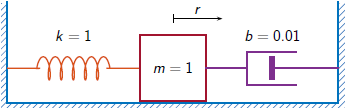
A one-dimensional discrete-time oscillating system consists of a unit mass, $m$ (in kg), attached to a wall by a spring with elastic constant $k = 1$ N/m. A sensor samples the displacement of the mass at $F_{s} = 1$ Hz. A damper impedes the motion of the mass by exerting on it a force proportional to speed, with damping constant $b = 0.01$ kg/s.

Mass-spring-damper system, with a mass of 1 kilogram, a spring with elastic constant k=1 Newton per meter, and a damper with damping constant b=0.01 kilograms per second. The displacement of the mass is r (in meters).

Generate 3000 time samples. Define the sampling interval $Δ t = 1 / F_{s}$ .

Fs = 1;
dt = 1/Fs;
N = 3000;
t = dt*(0:N-1);
b = 0.01;

The system can be described by the state-space model

$\begin{array}{c} x (k + 1) = A x (k) + B u (k), \\ y (k) = C x (k) + D u (k), \end{array}$

where $x = {[\begin{matrix} r & v \end{matrix}]}^{T}$ is the state vector, $r$ and $v$ are respectively the displacement and velocity of the mass, $u$ is the driving force, and $y = r$ is the measured output. The state-space matrices are

$A = \exp (A_{c} Δ t), B = A_{c}^{- 1} (A - I) B_{c}, C = [\begin{array}{c} 1 & 0 \end{array}], D = 0,$

$I$ is the $2 \times 2$ identity, and the continuous-time state-space matrices are

$A_{c} = [\begin{array}{c} 0 & 1 \\ - 1 & - b \end{array}], B_{c} = [\begin{array}{c} 0 \\ 1 \end{array}] .$

Ac = [0 1;-1 -b];
A = expm(Ac*dt);

Bc = [0;1];
B = Ac\(A-eye(2))*Bc;

C = [1 0];
D = 0;

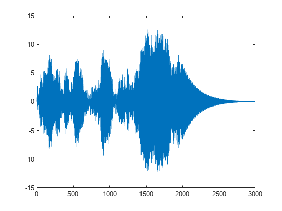
The mass is driven by random input for the first 2000 seconds and then left to return to rest. Use the state-space model to compute the time evolution of the system starting from an all-zero initial state. Plot the displacement of the mass as a function of time.

rng("default")
u = randn(1,N)/2;
u(2001:end) = 0;

y = 0;
x = [0;0];
for k = 1:N
    y(k) = C*x + D*u(k);
    x = A*x + B*u(k);
end

plot(t,y)

Figure contains an axes object. The axes object contains an object of type line.

Estimate the modal frequency-response function of the system. Use a Hann window half as long as the measured signals. Specify that the output is the displacement of the mass.

wind = hann(N/2);

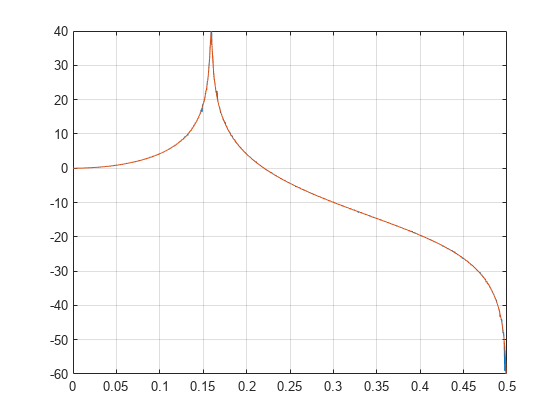
[frf,f] = modalfrf(u',y',Fs,wind,Sensor="dis");

The frequency-response function of a discrete-time system can be expressed as the Z-transform of the time-domain transfer function of the system, evaluated at the unit circle. Compare the modalfrf estimate with the definition.

[b,a] = ss2tf(A,B,C,D);

[ztf,fz] = freqz(b,a,2048,Fs);

plot(f,mag2db(abs(frf)))
hold on
plot(fz*Fs,mag2db(abs(ztf)))
hold off
grid
ylim([-60 40])

Figure contains an axes object. The axes object contains 2 objects of type line.

Estimate the natural frequency and the damping ratio for the vibration mode.

[fn,dr] = modalfit(frf,f,Fs,1,FitMethod="PP")

fn = 
0.1593

dr = 
0.0043

Compare the natural frequency to $1 / 2 π$ , which is the theoretical value for the undamped system.

theo = 1/(2*pi)

theo = 
0.1592

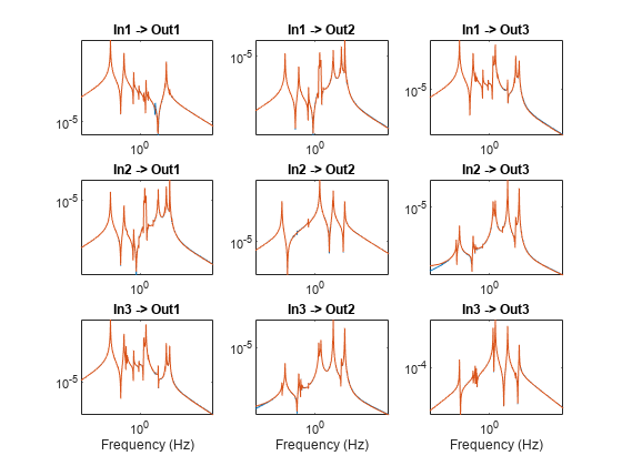
Modal Parameters Using Least-Squares Rational Function Method

Open Live Script

Compute the modal parameters of a Space Station module starting from its frequency-response function (FRF) array.

Load a structure containing the three-input/three-output FRF array. The system is sampled at 320 Hz.

load modaldata SpaceStationFRF

frf = SpaceStationFRF.FRF; 
f = SpaceStationFRF.f; 
fs = SpaceStationFRF.Fs;

Extract the modal parameters of the lowest 24 modes using the least-squares rational function method.

[fn,dr,ms,ofrf] = modalfit(frf,f,fs,24,'FitMethod','lsrf');

Compare the reconstructed FRF array to the measured one.

for ij = 1:3
 for ji = 1:3
    subplot(3,3,3*(ij-1)+ji)
    loglog(f,abs(frf(:,ji,ij)))
    hold on
    loglog(f,abs(ofrf(:,ji,ij)))
    hold off
    axis tight
    title(sprintf('In%d -> Out%d',ij,ji))
    if ij==3
        xlabel('Frequency (Hz)')
    end
 end
end

Modal Analysis of Two-Body Oscillator

Open Live Script

Estimate the modal parameters of a multi-input/multi-output (MIMO) system.

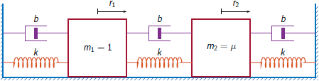
Two masses connected to a spring and a damper on each side form an ideal one-dimensional discrete-time oscillating system. The system input array u consists of random driving forces applied to the masses. The system output array y contains the observed displacements of the masses from their initial reference positions. The system is sampled at a rate Fs of 40 Hz.

Load the data file containing the MIMO system inputs, the system outputs, and the sample rate. The example Frequency-Response Analysis of MIMO System analyzes the system that generated the data used in this example.

load MIMOdata

Estimate the modal frequency response functions of the system. Use a 12000-sample Hann window with 9000 samples of overlap between adjoining segments. Specify the sensor data type as measured displacements.

wind = hann(12000);
nove = 9000;
[frf,f] = modalfrf(u,y,Fs,wind,nove,Sensor="dis");

Estimate the natural frequencies, damping ratios, and mode shapes of the system. Use two modes and pick the least-squares rational function estimation method for the calculation.

[fn,dr,ms] = modalfit(frf,f,Fs,2,FitMethod="lsrf")

ms = 2×2 complex

   0.0819 - 0.1139i   0.0016 - 0.0109i
   0.0442 - 0.0615i  -0.0602 + 0.2041i

Modal Parameters of MIMO System

Open Live Script

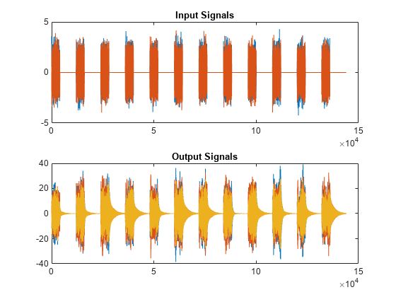
Compute the natural frequencies, the damping ratios, and the mode shapes for a two-input/three-output system excited by several bursts of random noise. Each burst lasts for 1 second, and there are 2 seconds between the end of each burst and the start of the next. The data are sampled at 4 kHz.

Load the data file. Plot the input signals and the output signals.

load modaldata

subplot(2,1,1)
plot(Xburst)
title('Input Signals')
subplot(2,1,2)
plot(Yburst)
title('Output Signals')

Figure contains 2 axes objects. Axes object 1 with title Input Signals contains 2 objects of type line. Axes object 2 with title Output Signals contains 3 objects of type line.

Compute the frequency-response functions. Specify a rectangular window with length equal to the burst period and no overlap between adjoining segments.

burstLen = 12000;
[frf,f] = modalfrf(Xburst,Yburst,fs,burstLen);

Visualize a stabilization diagram and return the stable natural frequencies. Specify a maximum model order of 30 modes.

figure
modalsd(frf,f,fs,'MaxModes',30);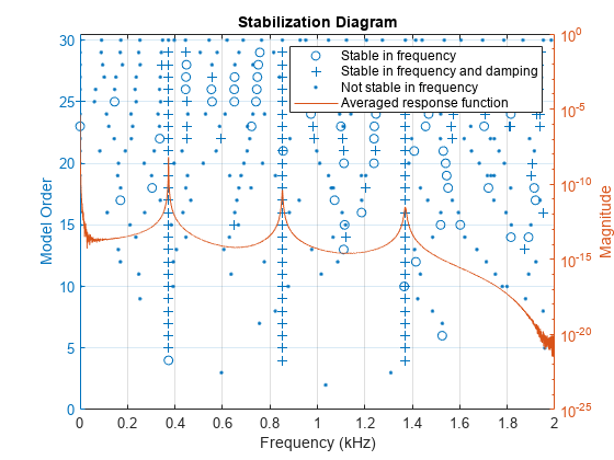

Figure contains an axes object. The axes object with title Stabilization Diagram, xlabel Frequency (kHz), ylabel Model Order contains 4 objects of type line. One or more of the lines displays its values using only markers These objects represent Stable in frequency, Stable in frequency and damping, Not stable in frequency, Averaged response function.

Zoom in on the plot. The averaged response function has maxima at 373 Hz, 852 Hz, and 1371 Hz, which correspond to the physical frequencies of the system. Save the maxima to a variable.

phfr = [373 852 1371];

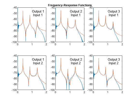
Compute the modal parameters using the least-squares complex exponential (LSCE) algorithm. Specify a model order of 6 modes and specify physical frequencies for the 3 modes determined from the stabilization diagram. The function generates one set of natural frequencies and damping ratios for each input reference.

[fn,dr,ms,ofrf] = modalfit(frf,f,fs,6,'PhysFreq',phfr);

Plot the reconstructed frequency-response functions and compare them to the original ones.

for k = 1:2
    for m = 1:3
        subplot(2,3,m+3*(k-1))
        plot(f/1000,10*log10(abs(frf(:,m,k))))
        hold on
        plot(f/1000,10*log10(abs(ofrf(:,m,k))))
        hold off
        text(1,-50,[['Output ';' Input '] num2str([m k]')])
        ylim([-100 -40])
    end
end
subplot(2,3,2)
title('Frequency-Response Functions')

Figure contains 6 axes objects. Axes object 1 contains 3 objects of type line, text. Axes object 2 with title Frequency-Response Functions contains 3 objects of type line, text. Axes object 3 contains 3 objects of type line, text. Axes object 4 contains 3 objects of type line, text. Axes object 5 contains 3 objects of type line, text. Axes object 6 contains 3 objects of type line, text.

Input Arguments

collapse all

`frf` — Frequency-response functions
vector | matrix | 3-D array

Frequency-response functions, specified as a vector, matrix, or 3-D array. frf has size p-by-m-by-n, where p is the number of frequency bins, m is the number of response signals, and n is the number of excitation signals used to estimate the transfer function. frf is assumed to be in dynamic flexibility (receptance) format.

Use modalfrf to generate a matrix of frequency-response functions from measured data.

Example: Undamped Harmonic Oscillator

The motion of a simple undamped harmonic oscillator of unit mass and elastic constant sampled at a rate $f_{s} = 1 / Δ t$ is described by the transfer function

$H (z) = \frac{N_{S e n s o r} (z)}{1 - 2 z^{- 1} \cos Δ t + z^{- 2}}$ ,

where the numerator depends on the magnitude being measured:

Displacement: $N_{d i s} (z) = (z^{- 1} + z^{- 2}) (1 - \cos Δ t)$
Velocity: $N_{v e l} (z) = (z^{- 1} - z^{- 2}) \sin Δ t$
Acceleration: $N_{a c c} (z) = (1 - z^{- 1}) - (z^{- 1} - z^{- 2}) \cos Δ t$

Compute the frequency-response function for the three possible system response sensor types. Use a sample rate of 2 Hz and 30,000 samples of white noise as input.

fs = 2;
dt = 1/fs;
N = 30000;

u = randn(N,1);

ydis = filter((1-cos(dt))*[0 1 1],[1 -2*cos(dt) 1],u);
[frfd,fd] = modalfrf(u,ydis,fs,hann(N/2),Sensor="dis");

yvel = filter(sin(dt)*[0 1 -1],[1 -2*cos(dt) 1],u);
[frfv,fv] = modalfrf(u,yvel,fs,hann(N/2),Sensor="vel");

yacc = filter([1 -(1+cos(dt)) cos(dt)],[1 -2*cos(dt) 1],u);
[frfa,fa] = modalfrf(u,yacc,fs,hann(N/2),Sensor="acc");

loglog(fd,abs(frfd),fv,abs(frfv),fa,abs(frfa))
grid
legend(["dis" "vel" "acc"],Location="best")

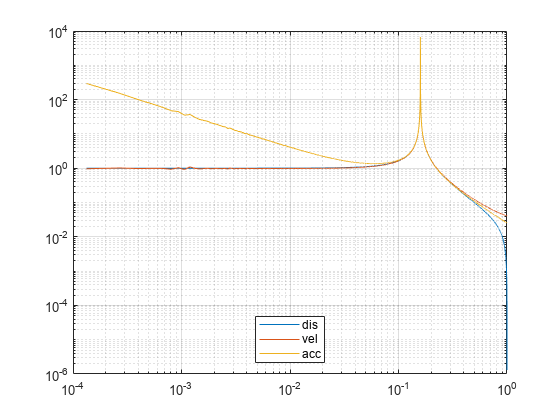
Figure contains an axes object. The axes object contains 3 objects of type line. These objects represent dis, vel, acc.

In all cases, the generated frequency-response function is in a format corresponding to displacement. Velocity and acceleration measurements are first and second time derivatives, respectively, of displacement measurements. The frequency-response functions are equivalent in the range around the natural frequency of the system. Away from the natural frequency, the frequency-response functions differ.

Data Types: single | double
Complex Number Support: Yes

`f` — Frequencies
vector

Frequencies, specified as a vector. The number of elements of f must equal the number of rows of frf.

Data Types: single | double

`fs` — Sample rate of measurement data
positive scalar

Sample rate of measurement data, specified as a positive scalar expressed in hertz.

Data Types: single | double

`mnum` — Number of modes
positive integer

Number of modes, specified as a positive integer.

Data Types: single | double

`sys` — Identified system
model with identified parameters

Identified system, specified as a model with identified parameters. Use estimation commands like ssest (System Identification Toolbox), n4sid (System Identification Toolbox), or tfest (System Identification Toolbox) to create sys starting from a measured frequency-response function or from time-domain input and output signals. See Modal Analysis of Identified Models for an example. You must have a System Identification Toolbox license to use this input argument.

Example: idss([0.5418 0.8373;-0.8373 0.5334],[0.4852;0.8373],[1 0],0,[0;0],[0;0],1) generates an identified state-space model corresponding to a unit mass attached to a wall by a spring of unit elastic constant and a damper with constant 0.01. The displacement of the mass is sampled at 1 Hz.

Example: idtf([0 0.4582 0.4566],[1 -1.0752 0.99],1) generates an identified transfer-function model corresponding to a unit mass attached to a wall by a spring of unit elastic constant and a damper with constant 0.01. The displacement of the mass is sampled at 1 Hz.

Name-Value Arguments

Specify optional pairs of arguments as Name1=Value1,...,NameN=ValueN, where Name is the argument name and Value is the corresponding value. Name-value arguments must appear after other arguments, but the order of the pairs does not matter.

Before R2021a, use commas to separate each name and value, and enclose Name in quotes.

Example: "FitMethod","pp",'FreqRange',[0 500] uses the peak-picking method to perform the fit and restricts the frequency range to between 0 and 500 Hz.

`Feedthrough` — Presence of feedthrough in estimated transfer function
`false` (default) | `true`

Presence of feedthrough in estimated transfer function, specified as a logical value. This argument is available only if 'FitMethod' is specified as "lsrf".

Data Types: logical

`FitMethod` — Fitting algorithm
`"lsce"` (default) | `"lsrf"` | `"pp"`

Fitting algorithm, specified as "lsce", "lsrf", or "pp".

"lsce" — Least-Squares Complex Exponential Method. If you specify "lsce", then fn is a vector with mnum elements, independent of the size of frf.
"lsrf" — Least-squares rational function estimation method. If you specify "lsrf", then fn is a vector with mnum elements, independent of the size of frf. The method is described in [3]. See Continuous-Time Transfer Function Estimation Using Continuous-Time Frequency-Domain Data (System Identification Toolbox) for more information. This algorithm typically requires less data than nonparametric approaches and is the only one that works for nonuniform f.
"pp" — Peak-Picking Method. For an frf computed from n excitation signals and m response signals, fn is an mnum-by-m-by-n array with one estimate of fn and one estimate of dr per frf.

`FreqRange` — Frequency range
two-element vector of increasing positive values

Frequency range, specified as a two-element vector of increasing positive values contained within the range specified in f.

Data Types: single | double

`PhysFreq` — Natural frequencies for physical modes
vector

Natural frequencies for physical modes to include in the analysis, specified as a vector of frequency values within the range spanned by f. The function includes in the analysis those modes with natural frequencies closest to the values specified in the vector. If the vector contains m frequency values, then fn and dr have m rows each, and ms has m columns. If you do not specify this argument, then the function uses the entire frequency range in f.

Data Types: single | double

`DriveIndex` — Indices of the driving-point frequency-response function
`[1 1]` (default) | two-element vector of positive integers

Indices of the driving-point frequency-response function, specified as a two-element vector of positive integers. The first element of the vector must be less than or equal to the number of system responses. The second element of the vector must be less than or equal to the number of system excitations. Mode shapes are normalized to unity modal based on the driving point.

Example: "DriveIndex",[2 3] specifies that the driving-point frequency-response function is frf(:,2,3).

Data Types: single | double

Output Arguments

collapse all

`fn` — Natural frequencies
matrix | 3-D array

Natural frequencies, returned as a matrix or 3-D array. The size of fn depends on the choice of fitting algorithm specified with 'FitMethod':

If you specify "lsce" or "lsrf", then fn is a vector with mnum elements, independent of the size of frf. If the system has more than mnum oscillatory modes, then the "lsrf" method returns the first mnum least-damped modes sorted in order of increasing natural frequency.
If you specify "pp", then fn is an array of size mnum-by-m-by-n with one estimate of fn and one estimate of dr per frf.

`dr` — Damping ratios
matrix | 3-D array

Damping ratios for the natural frequencies in fn, returned as a matrix or 3-D array of the same size as fn.

`ms` — Mode-shape vectors
matrix

Mode-shape vectors, returned as a matrix. ms has mnum columns, each containing a mode-shape vector of length q, where q is the larger of the number of excitation channels and the number of response channels.

`ofrf` — Reconstructed frequency-response functions
vector | matrix | 3-D array

Reconstructed frequency-response functions, returned as a vector, matrix, or 3-D array with the same size as frf.

Algorithms

collapse all

Least-Squares Complex Exponential Method

The least-squares complex exponential method computes the impulse response corresponding to each frequency-response function and fits to the response a set of complex damped sinusoids using Prony’s method.

A sampled damped sinusoid can be cast in the form

$\begin{matrix} s_{i} (n) = A_{i} e^{- b_{i} n / f_{s}} \cos (2 π f_{i} n / f_{s} + ϕ_{i}) \\ = \frac{1}{2} A_{i} e^{j ϕ_{i}} \exp (- (b_{i} / f_{s} - j 2 π f_{i} / f_{s}) n) + \frac{1}{2} A_{i} e^{- j ϕ_{i}} \exp (- (b_{i} / f_{s} + j 2 π f_{i} / f_{s}) n) \\ \equiv a_{i +} x_{i +}^{n} + a_{i -} x_{i -}^{n}, \end{matrix}$

where:

f_s is the sample rate.
f_i is the sinusoid frequency.
b_i is the damping coefficient.
A_i and ϕ_i are the amplitude and phase of the sinusoid.

The a_i are called amplitudes and the x_i are called poles. Prony’s method expresses a sampled function h(n) as a superposition of N/2 modes (and thus N amplitudes and poles):

$\begin{matrix} h (0) = a_{1} x_{1}^{0} + a_{2} x_{2}^{0} \dots + a_{N} x_{N}^{0} \\ h (1) = a_{1} x_{1}^{1} + a_{2} x_{2}^{1} + \dots + a_{N} x_{N}^{1} \\ ⋮ \\ h (N - 1) = a_{1} x_{1}^{N - 1} + a_{2} x_{2}^{N - 1} + \dots + a_{N} x_{N}^{N - 1} . \end{matrix}$

The poles are the roots of a polynomial with coefficients c₀, c₁, …, c_N–1:

$x_{i}^{N} + c_{N - 1} x_{i}^{N - 1} + \dots + c_{1} x_{i}^{1} + c_{0} x_{i}^{0} = 0.$

The coefficients are found using an autoregressive model of L = 2N samples of h:

$[\begin{matrix} h (0) & h (1) & \dots & h (N - 1) \\ h (1) & h (2) & \dots & h (N) \\ ⋮ & ⋮ & ⋱ & ⋮ \\ h (L - N - 1) & h (L - N) & \dots & h (L - 2) \end{matrix}] [\begin{matrix} c_{0} \\ c_{1} \\ ⋮ \\ c_{N - 1} \end{matrix}] = - [\begin{matrix} h (N) \\ h (N + 1) \\ ⋮ \\ h (L - 1) \end{matrix}] .$

To find the poles, the algorithm uses the roots function. Once the poles are known, it is possible to determine the frequencies and damping factors by identifying the imaginary and real parts of the pole logarithms. The final step is solving for the amplitudes and reconstructing the impulse response using

$[\begin{matrix} h (0) \\ ⋮ \\ h (N - 1) \end{matrix}] = [\begin{matrix} x_{1}^{0} & \dots & x_{N}^{0} \\ ⋮ & ⋱ & ⋮ \\ x_{1}^{N - 1} & \dots & x_{N}^{N - 1} \end{matrix}] [\begin{matrix} a_{1} \\ ⋮ \\ a_{N} \end{matrix}] .$

The following naive MATLAB^® implementation summarizes the procedure:

N = 4;
L = 2*N;
h = rand(L,1);
c = hankel(h(1:N),h(L-N:L-1))\-h(N+1:L);
x = roots([1;c(N:-1:1)]).';
p = log(x);
hrec = x.^((0:L-1)')*(x.^((0:L-1)')\h(1:L));
sum(h-hrec)

ans =

   3.2613e-15 - 1.9297e-16i

The system can also be constructed to contain samples from multiple frequency-response functions and solved using least squares.

Peak-Picking Method

The peak-picking method assumes that each significant peak in the frequency-response function corresponds to exactly one natural mode. Close to a peak, the system is assumed to behave like a one-degree-of-freedom damped harmonic oscillator:

$H (f) = \frac{- 1}{{(2 π)}^{2}} \frac{1 / m}{f^{2} - j 2 ζ_{r} f_{r} f - f_{r}^{2}} \Rightarrow f_{r}^{2} H (f) + j 2 ζ_{r} f_{r} f H (f) - \frac{1}{{(2 π)}^{2} m} = f^{2} H (f),$

where H is the frequency-response function, f_r is the undamped resonance frequency, ζ_r = b/(4mk)^1/2 is the relative damping, b is the damping constant, k is the elastic constant, and m is the mass.

Given a peak located at f_p, the procedure takes the peak and a fixed number of points to either side, replaces the mass term with a dummy variable, d, and computes the modal parameters by solving the system of equations

$[\begin{matrix} H (f_{p - k}) & j 2 f_{p - k} H (f_{p - k}) & - 1 \\ ⋮ & ⋮ & ⋮ \\ H (f_{p}) & j 2 f_{p} H (f_{p}) & - 1 \\ ⋮ & ⋮ & ⋮ \\ H (f_{p + k}) & j 2 f_{p + k} H (f_{p + k}) & - 1 \end{matrix}] [\begin{matrix} f_{r}^{2} \\ ζ_{r} f_{r} \\ d \end{matrix}] = [\begin{matrix} f_{p - k}^{2} H (f_{p - k}) \\ ⋮ \\ f_{p}^{2} H (f_{p}) \\ ⋮ \\ f_{p + k}^{2} H (f_{p + k}) \end{matrix}] .$

References

[1] Allemang, Randall J., and David L. Brown. “Experimental Modal Analysis and Dynamic Component Synthesis, Vol. III: Modal Parameter Estimation.” Technical Report AFWAL-TR-87-3069. Air Force Wright Aeronautical Laboratories, Wright-Patterson Air Force Base, OH, December 1987.

[2] Brandt, Anders. Noise and Vibration Analysis: Signal Analysis and Experimental Procedures. Chichester, UK: John Wiley & Sons, 2011.

[3] Ozdemir, Ahmet Arda, and Suat Gumussoy. "Transfer Function Estimation in System Identification Toolbox via Vector Fitting." Proceedings of the 20th World Congress of the International Federation of Automatic Control, Toulouse, France, July 2017.

Extended Capabilities

C/C++ Code Generation
Generate C and C++ code using MATLAB® Coder™.

Usage notes and limitations:

Identified system model inputs are not supported for code generation.
The "lsrf" fitting algorithm is not supported for code generation.

Version History

Introduced in R2017a

expand all

R2024b: `modalfit` supports C/C++ code generation

The modalfit function supports C/C++ code generation. You must have MATLAB Coder™ to use this functionality.

modalfit

Syntax

Description

Examples

Frequency-Response Function of SISO System

Modal Parameters Using Least-Squares Rational Function Method

Modal Analysis of Two-Body Oscillator

Modal Parameters of MIMO System

Input Arguments

`frf` — Frequency-response functions
vector | matrix | 3-D array

Example: Undamped Harmonic Oscillator

`f` — Frequencies
vector

`fs` — Sample rate of measurement data
positive scalar

`mnum` — Number of modes
positive integer

`sys` — Identified system
model with identified parameters

Name-Value Arguments

`Feedthrough` — Presence of feedthrough in estimated transfer function
`false` (default) | `true`

`FitMethod` — Fitting algorithm
`"lsce"` (default) | `"lsrf"` | `"pp"`

`FreqRange` — Frequency range
two-element vector of increasing positive values

`PhysFreq` — Natural frequencies for physical modes
vector

`DriveIndex` — Indices of the driving-point frequency-response function
`[1 1]` (default) | two-element vector of positive integers

Output Arguments

`fn` — Natural frequencies
matrix | 3-D array

`dr` — Damping ratios
matrix | 3-D array

`ms` — Mode-shape vectors
matrix

`ofrf` — Reconstructed frequency-response functions
vector | matrix | 3-D array

Algorithms

Least-Squares Complex Exponential Method

Peak-Picking Method

References

Extended Capabilities

C/C++ Code Generation
Generate C and C++ code using MATLAB® Coder™.

Version History

R2024b: `modalfit` supports C/C++ code generation

See Also

Topics

modalfit

Syntax

Description

Examples

Frequency-Response Function of SISO System

Modal Parameters Using Least-Squares Rational Function Method

Modal Analysis of Two-Body Oscillator

Modal Parameters of MIMO System

Input Arguments

frf — Frequency-response functions vector | matrix | 3-D array

Example: Undamped Harmonic Oscillator

f — Frequencies vector

fs — Sample rate of measurement data positive scalar

mnum — Number of modes positive integer

sys — Identified system model with identified parameters

Name-Value Arguments

Feedthrough — Presence of feedthrough in estimated transfer function false (default) | true

FitMethod — Fitting algorithm "lsce" (default) | "lsrf" | "pp"

FreqRange — Frequency range two-element vector of increasing positive values

PhysFreq — Natural frequencies for physical modes vector

DriveIndex — Indices of the driving-point frequency-response function [1 1] (default) | two-element vector of positive integers

Output Arguments

fn — Natural frequencies matrix | 3-D array

dr — Damping ratios matrix | 3-D array

ms — Mode-shape vectors matrix

ofrf — Reconstructed frequency-response functions vector | matrix | 3-D array

Algorithms

Least-Squares Complex Exponential Method

Peak-Picking Method

References

Extended Capabilities

C/C++ Code Generation Generate C and C++ code using MATLAB® Coder™.

Version History

R2024b: modalfit supports C/C++ code generation

See Also

Topics

`frf` — Frequency-response functions
vector | matrix | 3-D array

`f` — Frequencies
vector

`fs` — Sample rate of measurement data
positive scalar

`mnum` — Number of modes
positive integer

`sys` — Identified system
model with identified parameters

`Feedthrough` — Presence of feedthrough in estimated transfer function
`false` (default) | `true`

`FitMethod` — Fitting algorithm
`"lsce"` (default) | `"lsrf"` | `"pp"`

`FreqRange` — Frequency range
two-element vector of increasing positive values

`PhysFreq` — Natural frequencies for physical modes
vector

`DriveIndex` — Indices of the driving-point frequency-response function
`[1 1]` (default) | two-element vector of positive integers

`fn` — Natural frequencies
matrix | 3-D array

`dr` — Damping ratios
matrix | 3-D array

`ms` — Mode-shape vectors
matrix

`ofrf` — Reconstructed frequency-response functions
vector | matrix | 3-D array

C/C++ Code Generation
Generate C and C++ code using MATLAB® Coder™.

R2024b: `modalfit` supports C/C++ code generation