Practical Introduction to Shock Waveform and Shock Response Spectrum

Open Live Script

This example shows how to compute shock response spectra of synthetic and measured transient acceleration signals. The shock response spectrum (SRS) is a graphical representation of how various single-degree-of-freedom systems react to a transient acceleration input. SRS is commonly used to determine the frequency response of shock environments and to estimate the maximum dynamic response of structures. Additionally, SRS is utilized as a tool for designing specifications to characterize impulsive loads such as earthquakes, underwater explosions, stage separation forces, and pyrotechnic events.

Transient Data and Transient Analysis

An input to a system is considered transient if the input parameters change faster that the system time scale [1]. Suppose that the output of an oscillator is fed to a second-order filter resonant at 100 Hz. Let the amplitude change linearly by some factor $A$ in a time interval $T$ . If $T$ is 10 minutes, the output at any time during this period can be accurately predicted. The output is a sine wave of the same frequency as the input, and its magnitude varies linearly with time by the same factor $A$ . If, on the other hand, the change in level occurs in 1 millisecond, transient analysis techniques must be used to predict the output during the change and shortly thereafter. Thus, the classification of a particular time history as transient depends on how the system of interest responds to this time history. Mechanical shocks are usually of great interest in the design and operation of physical systems because the instantaneous input levels are larger than the steady-state inputs by an order of magnitude or more.

The ultimate goal of transient analysis is the determination of the damage potential of a shock upon a physical system [1]. The objective is to design the system to survive the shock environment or to attenuate the shock input to the system using packaging or attenuation devices. Survival of a shock excitation can mean one of two things:

The system exhibits no permanent damage after the shock
The system exhibits no degradation of performance either during or after the shock

As an example of the first definition, consider a microwave oven that has been accidentally dropped on the floor. Whether the microwave functions properly during the drop is of no concern. Even if calibration has to be performed after the drop, it is of no concern as long as the microwave is not permanently damaged by the fall and continues to function. As an example of the second definition, consider the launching of a satellite. If the shock that occurs in the satellite's body structure due to the separation of the satellite from the rocket in space causes even a brief malfunction of the onboard systems, the satellite will fail to propel itself to orbit and complete its mission. In this case, the system is not damaged permanently yet fails the second definition of survival.

The design of a system that withstands its shock environment requires the definition of this environment with reasonable accuracy because survival is not the only design factor. For example, weight and size are also frequently important and, yet, usually inversely related to the shock resistance of a system. The strength of a system is usually weight-dependent, while the packaging of the system to reduce shock input is usually size-dependent. However, in many applications, size and weight must be minimized, for example, in space applications where small weight increases require large increases in booster performance. Thus, the system must be able to withstand the shock environment but cannot have a large safety factor because of the weight restriction.

Shock Waveform

Shock refers to the sudden modification of a force, position, velocity, or acceleration resulting in a temporary state change of the considered system. This modification is deemed abrupt if it occurs within a period that is significantly shorter than the relevant system's natural period, as defined in [2], [3], [4]. Shock is characterized as a vibration that persists for a duration ranging between the natural period of the stimulated mechanical system and twice the natural period. The measurement of shock involves tracing the value of a shock parameter over time during the shock's duration, which is referred to as a time history [3].

A shock that can be precisely expressed in uncomplicated mathematical equations is known as a simple or perfect shock [3]. A general simple shock waveform can be expressed as [5],[6]

$s_{g} (t) = {\begin{cases} A {(\frac{t}{τ})}^{+ ζ ω τ} e^{- ζ ω (t - τ) + j (ω t + φ)} u (t), & τ \geq 0 \\ A {(\frac{t}{τ})}^{- ζ ω τ} e^{+ ζ ω (t - τ) + j (ω t + φ)} (1 - u (t)), & τ < 0 \end{cases}$

where $ω$ is the resonant frequency of the carrier wave, $ζ$ denotes the damping ratio which influences the duration of the shock waveform, and

$τ$ denotes the duration between the initial time and the peak time
$A$ is the maximum of the envelope curve
$φ$ is the phase
$u (t)$ is the unit step signal: $u (t) = 1$ for $t > 0$ and 0 otherwise

The shock waveform expressed above can be considered an amplitude-modulated harmonic waveform. This figure shows the time history and spectrum of a general simple shock with $φ = π ⌊ \frac{τ ω}{π} ⌋ - τ ω$ where $⌊ \cdot ⌋$ denotes the floor function.

generalShockWaveformParams = struct( ...
    "SampleRate",1e5, ...                                   % Hz
    "MaxEnvelope",9.81, ...                                 % m/s^2
    "CarrierFrequency",2000, ...                            % Hz
    "DampingRatio",2.5, ...
    "PeakTime",0.01, ...                                    % s
    "Phase",pi*floor(0.01*2*pi*2000/pi)-0.01*2*pi*2000, ... % rad
    "Duration",0.02 ...                                     % s
    );
plotGeneralSimpleShockWaveform(generalShockWaveformParams)

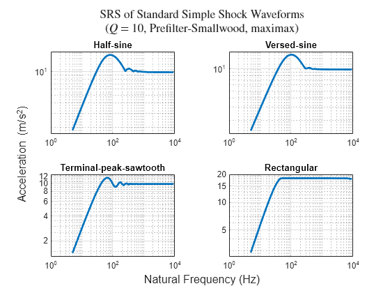
Standards typically define four simple shock waveforms:

Half-sine shock: $s_{hs} (t) = a \sin (\frac{π}{T_{0}} t)$ if $t \in [0, T_{0}]$ and $0$ if $t \in (T_{0}, T]$
Versed sine (or haversine) shock: $s_{vs} (t) = \frac{a}{2} [1 - \cos (\frac{2 π}{T_{0}} t)]$ if $t \in [0, T_{0}]$ and $0$ if $t \in (T_{0}, T]$
Terminal peak sawtooth shock: $s_{tps} (t) = a \frac{t}{T_{0}}$ if $t \in [0, T_{0}]$ and $0$ if $t \in (T_{0}, T]$
Rectangular shock waveform: $s_{rect} (t) = a$ if $t \in [0, T_{0}]$ and $0$ if $t \in (T_{0}, T]$

where $a$ , $T_{0}$ , and $T$ denote the amplitude, duty cycle, and duration of the waveform, respectively. The figure below displays these four simple shock waveforms, each of which has a duty cycle of 10 milliseconds, a duration of 20 milliseconds, and an amplitude of 9.81 meters/second $^{2}$ .

simpleShockWaveformParams = struct( ...
    "SampleRate",1e5, ... Hz
    "Amplitude",9.81, ... m/s^2
    "DutyCycle",1e-2, ... s
    "Duration",2e-2   ... s
    );
plotStandardSimpleShockWaveforms(simpleShockWaveformParams)

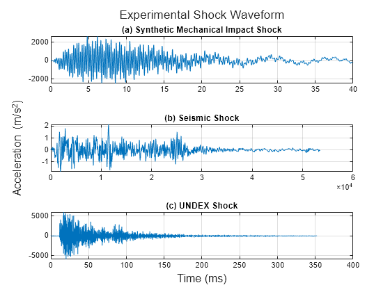
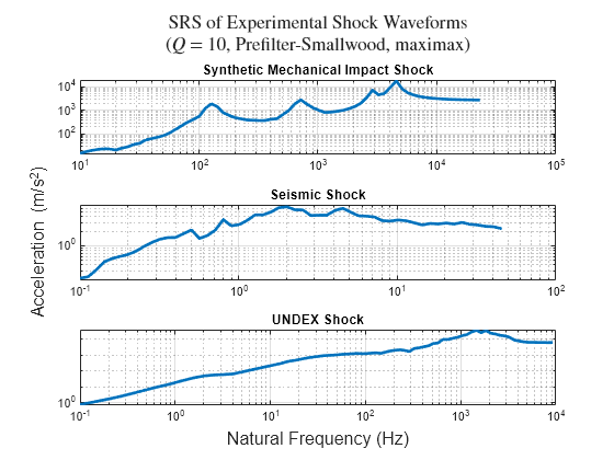
The shock waveforms that occur in the real world do not lend themselves to be expressed in closed form expression. This figure displays (a) a far-field metal-metal mechanical-impact shock that is synthesized using the general shock waveform expression and the parameters in [5], (b) a real world transient seismic shock waveform [7], and (c) an experimental underwater explosive (UNDEX) shock [8].

plotExperimentalShockWaveform

Shock Response Spectrum

The response of a system to a shock can be expressed as a temporal evolution of a parameter, such as displacement, velocity, or acceleration, that characterizes the motion of the system. The most common parameter is acceleration. For a simple system, the acceleration response peak amplitudes are a function of the system's natural frequency or natural period at different critical damping ratios. This representation is known as a shock response spectrum (SRS), response spectrum, or shock spectrum [3]. Biot developed the shock spectrum as a technique for approximating the destructive effects of seismic shocks on buildings, and it has since been utilized to analyze shocks applied to many linear systems.

The design of equipment and components used in aerospace, transportation, defense, and package engineering must account for the shock environment. The shock spectrum is employed to determine if a system can survive a shock environment, design the system to withstand shock environments, and specify shock tests [1]. The shock spectrum enables the characterization of the shock effect on a standardized dynamical system to estimate its severity or destructive potential and therefore enables comparison of different shocks or the establishment of equivalence criteria between a measured transient environment and a laboratory simulation of that environment [9]. Engineers can use SRS data to create durable spacecraft, avionics components, and electronic gadgets that can withstand anticipated shock environments. For example, a hardware design engineer can adjust the natural frequency of the component to reduce the peak response by modifying the design of the component.

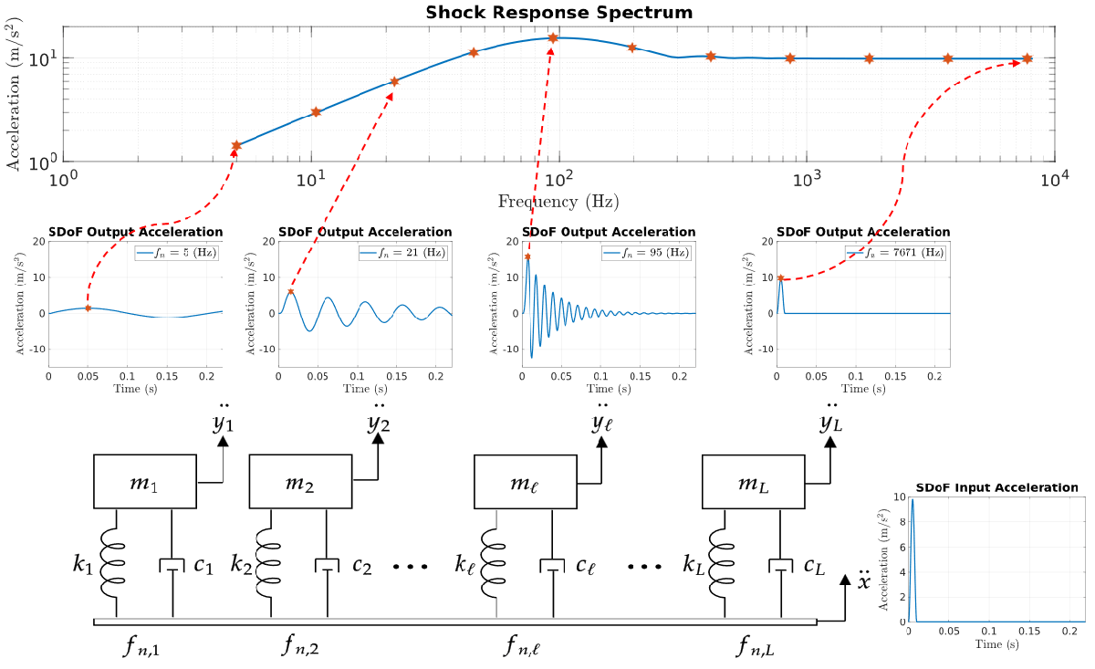
The SRS is a graph that illustrates the variations in the maximum responses of a set of linear single-degree-of-freedom (SDoF) systems that undergo mechanical excitation. These variations are plotted against the natural frequencies of these systems that usually have the same damping ratio value. By focusing on the response of a linear, viscously damped SDoF system with lumped parameters, only two parameters determine the response: (1) the undamped natural frequency and (2) the fraction of critical damping or resonant gain. Since only two parameters are involved, it is possible to obtain a systematic presentation of the peak responses of many simple structures from the shock measurement. This process is known as data reduction to the response domain [3].

The figure below provides a qualitative graphical representation of the construction of a shock response spectrum. It depicts a transient acceleration-time history input applied to a base on which a series of linear oscillators of different natural frequencies are mounted. The base is assumed to be massive enough that the motion of the oscillators does not affect its motion and there is no coupling between masses and the base. The transient acceleration response of each oscillator is shown graphically above each oscillator. In this case, oscillator 1 has the lowest frequency and lower maximum acceleration amplitude and oscillator $ℓ$ has the highest maximum response relative to the others. As the frequency increases to the right, the maximum acceleration response decreases. The SRS graph at the top of the figure is used to characterize the frequency content of the transient shock input signal. The maximum response drops off for systems of higher and lower frequencies, representing stiffer and softer systems, respectively.

Response of a Linear Single-Degree-of-Freedom System

To construct the SRS graph, compute the response of each SDoF oscillator to the base acceleration. This figure illustrates such a linear SDoF oscillator subjected to an input acceleration $x_{}^{¨} (t)$ .

In this figure, $m$ , $k$ , and $c$ denote the mass, stiffness of the spring, and viscous damping coefficient of the oscillator, respectively, and $y_{}^{¨} (t)$ is the absolute acceleration response of the SDoF oscillator. To obtain the response of an SDoF oscillator under a given base input, solve the equation of motion

$z_{}^{¨} (t) + \frac{ω_{n}}{Q} z_{}^{˙} (t) + ω_{n}^{2} z (t) = - x_{}^{¨} (t)$

where $z (t) = y (t) - x (t)$ is the relative displacement of the mass, $Q = \frac{\sqrt{k m}}{c}$ is the quality factor, and $ω_{n} = 2 π f_{n} = \sqrt{\frac{k}{m}}$ is the natural angular frequency. If the initial relative displacement and velocity of the system are both zero, the solution to the equation of motion is given by the convolution of $- x_{}^{¨} (t)$ with the unit impulse response of the SDoF system

$z (t) = - \frac{1}{ω_{d}} \int_{0}^{t} x_{}^{¨} (τ) e^{- ζ ω_{n} (t - τ)} \sin (ω_{d} (t - τ)) d τ$ ,

where $ζ = \frac{1}{2 Q}$ is the damping ratio and $ω_{d} = ω_{n} \sqrt{1 - ζ^{2}}$ denotes the damped natural angular frequency. The solution in terms of the absolute acceleration $y_{}^{¨} (t)$ is $y_{}^{¨} (t) = - 2 ζ ω_{n} z_{}^{˙} (t) - ω_{n}^{2} z (t)$ . In this example, the absolute acceleration response is used to compute the response spectrum.

Algorithms to Compute Shock Response Spectra

There are four common discrete-time methods that can be used to compute the absolute acceleration response.

Recursive integration method: In this method, the solution for $z_{k}$ and ${z_{}^{˙}}_{k}$ (where $x_{k} = x (t_{k})$ ) are treated as initial conditions in calculating $z_{k + 1}$ and ${z_{}^{˙}}_{k + 1}$ . The integrals to compute $z (t)$ and $z_{}^{˙} (t)$ only need to be evaluated over $τ \in [0, Δ t]$ , where $Δ t = t_{k + 1} - t_{k}$ is the regular sample time. Use a parabolic approximation to compute the integrals [1], [10].

Recursive filtering method: This method uses impulse invariance to convert the continuous-time transfer function $H (s) = \frac{2 ζ ω_{n} s + ω_{n}^{2}}{s^{2} + 2 ζ ω_{n} s + ω_{n}^{2}}$ to the digital filter with $H (z) = \frac{b_{0} + b_{1} z^{- 1}}{1 + a_{1} z^{- 1} + a_{2} z^{- 2}}$ where $a_{1} = - 2 e^{- ζ ω_{n} Δ t} \cos (ω_{d} Δ t)$ , $a_{2} = e^{- 2 ζ ω_{n} Δ t}$ , $b_{0} = 2 ζ ω_{n} Δ t$ , and

$b_{1} = ω_{n} Δ t (\frac{ω_{n}}{ω_{d}} (1 - 2 ζ^{2}) e^{- ζ ω_{n} Δ t} \sin (ω_{d} Δ t) - 2 ζ e^{- ζ ω_{n} Δ t} \cos (ω_{d} Δ t)) .$

Smallwood method: This method uses ramp invariance to convert the transfer function to an equivalent digital filter with unit DC response [11]. Ramp invariance connects impulse-response samples with straight lines to decrease aliasing. Aliasing is the main reason that the digital filter obtained from the impulse-invariant method does not have a unit DC response.

Prefilter-Smallwood method: This method improves on the previous one by using an optimized lowpass pre-filter to remove the distortion caused by the straight-line connections [12].

The function hSrs implements the four methods.

Natural Frequencies and Damping Ratio

As mentioned earlier, only two parameters are required to construct an SRS graph: (1) natural frequency $f_{n}$ and (2) damping ratio $ζ$ , or equivalently quality factor $Q$ .

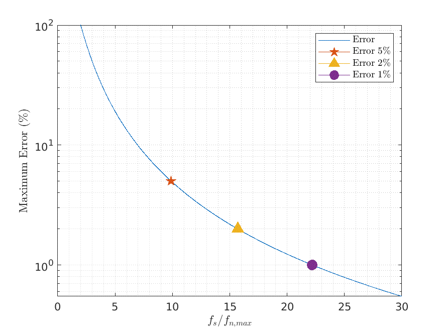
The set of natural frequencies in the shock spectrum is bounded by the sample rate of the acceleration signals. There is a bias error in detecting true peaks in the sampled acceleration response which is in general calculated with the same temporal step as that of the input shock acceleration. If the response is a sinusoid, which is the case for zero damping, then the maximum error in finding the true peak is bounded by $1 - \cos (π / M)$ , where $M$ denotes the ratio of the sample rate $f_{s}$ to the maximum natural frequency $f_{n, max}$ [2]. Therefore, the sample rate must be higher than 10 times the maximum frequency of the spectrum so that the error made at high frequencies is lower than 5%. For a maximum error of 1%, the sample rate should be higher than 23 times the maximum frequency of the spectrum as shown in the figure [3].

It is usually quite difficult to determine the true damping of the system. In practice, the shock response spectrum is calculated at several different critical damping ratio values in the range of 0 to 0.1 (from undamped to 10 percent of critical damping). A typical value of the damping ratio is 0.05, which is equivalent to a quality factor $Q = 10$ .

In the figure below, the SRS of a rectangular shock waveform of the duty cycle of 10 milliseconds, duration of 20 milliseconds, and amplitude of 9.81 meters/second $^{2}$ is computed using the three methods. The sample rate is 100 kHz and the natural frequencies at which the SRS is computed belong to the interval [5, 10,000] Hz. For this specific waveform, the recursive integration method suffers from numerical approximation error in higher natural frequencies. To reduce the error of the recursive integration approach and achieve the same SRS curve as the ones obtained by the other three methods, the rectangular waveform must be discretized at higher sample rate like 500 kHz.

simpleShockWaveformName = "Rectangular";
plotSRSMethods(simpleShockWaveformName,simpleShockWaveformParams)

When dealing with high frequencies, it is important to note that the shock spectrum level approaches the maximum base acceleration. The understanding of this behavior can be aided by looking at the free-body diagram of an SDoF oscillator. Typically, when acceleration is applied to the base of this oscillator, the acceleration of the mass is amplified, as seen in the middle region of the figure. However, if the oscillator has a high frequency and a relatively stiff spring compared to the mass, it behaves like a rigid body relative to the base. This means that the spring does not compress or extend and the base acceleration is directly transmitted to the mass. Therefore, the mass accelerations are the same as the base accelerations, including the maxima [4].

Spectrum Type

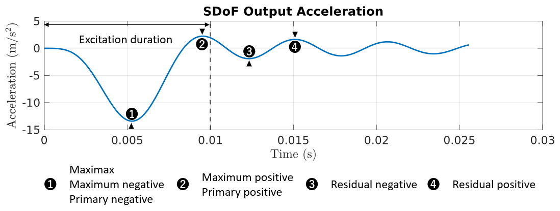
Several different shock response spectra can be constructed from a single transient response depending on which feature of the transient is selected. These types for one frequency are illustrated in the response time history shown in the figure. They may be classified by the polarity of the peak response and its time of occurrence. The maximax spectrum consists of the maximum absolute response recorded as a function of natural frequency of the system. The maximum positive spectrum contains only the maximum positive response excursions, while the maximum negative spectrum contains only the maximum negative excursions. The primary spectrum is made up of the maximum absolute responses during the excitation, while the residual spectrum contains the peak response occurring after the excitation has decayed completely.

This figure illustrates the three types of shock response spectra for a terminal-peak-sawtooth shock waveform with a duty cycle of 10 milliseconds, a duration of 20 milliseconds, and an amplitude of 9.81 meter/second $^{2}$ .

simpleShockWaveformName = "Terminal-peak-sawtooth";
plotSRSSpectrumTypes(simpleShockWaveformName,simpleShockWaveformParams)

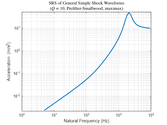
Examples of Shock Response Spectra

This section displays the SRS for the general waveform, the four standard waveforms, and the four experimental waveforms, computed using these parameters:

Q = 10;
method = "Prefilter-Smallwood";
spectrumType = "maximax";

General Simple Shock Waveform

plotGeneralShockSRS(Q,method,spectrumType,generalShockWaveformParams)

Standard Simple Shock Waveform

plotSimpleShockSRS(Q,method,spectrumType,simpleShockWaveformParams)

Experimental Shock Waveform

plotExperimentalShockSRS(Q,method,spectrumType)

Conclusion

In this example, we introduced the concept of shock response spectrum, surveyed different types of SRS, and discussed how to use the SRS to design a component or specify test requirements. We also talked about how to compute shock response spectra and implemented four methods to obtain SRS. We demonstrated the methods using both simulated and experimental signals and discussed how to choose natural frequencies based on the sample rate of the input acceleration-time history.

Acknowledgement

Seismic shock data [7] is obtained from the strong-motion data. Strong-motion data was accessed through the Center for Engineering Strong Motion Data (CESMD), last visited on July 5, 2023. The networks or agencies providing the data used in this report are the California Strong Motion Instrumentation Program (CSMIP) and the USGS National Strong Motion Project (NSMP).

References

[1] Kelly, Ronald D., and George Richman. “Principles and Techniques of Shock Data Analysis.” Washington: Naval Research Laboratory, 1969.

[2] Lalanne, Christian. Mechanical Vibration and Shock Analysis. Vol. 2: Mechanical Shock / Christian Lalanne. 2. ed. Vol. 2. London: ISTE, 2009.

[3] Piersol, Allan G., Thomas L. Paez, and Cyril M. Harris. Harris’ Shock and Vibration Handbook. 6th ed. New York: McGraw-Hill, 2010.

[4] Alexander, J. Edward. “Shock Response Spectrum-a Primer.” Sound and Vibration 43 (2009): 6–15.

[5] Yan, Yinzhong, and Q.M. Li. “A General Shock Waveform and Characterisation Method.” Mechanical Systems and Signal Processing 136 (February 2020): 106508. https://doi.org/10.1016/j.ymssp.2019.106508.

[6] Yan, Yinzhong, and Q.M. Li. “Effective Waveform Representation of Responsive Signals Initiated by Impulsive Actions in Physical and Engineering Systems.” International Journal of Engineering Science 147 (February 2020): 103199. https://doi.org/10.1016/j.ijengsci.2019.103199.

[7] COSMOS Virtual Data Center. “El Centro 1940-05-19 04:36:41 UTC - Component: 270,” May 1940. https://www.strongmotioncenter.org/vdc/scripts/event.plx?evt=88.

[8] enDAQ. “Shock Analysis: Response Spectrum (SRS), Pseudo Velocity & Severity.” EnDAQ. EnDAQ Blog (blog), 2020. https://blog.endaq.com/shock-analysis-response-spectrum-srs-pseudo-velocity-severity.

[9] European Cooperation for Space Standardization. Mechanical Shock Design and Verification Handbook. Noordwijk, The Netherlands: ESA Requirements and Standards Division, 2015.

[10] Martin, Justin N., Andrew J. Sinclair, and Winfred A. Foster. “On the Shock-Response-Spectrum Recursive Algorithm of Kelly and Richman.” Shock and Vibration 19, no. 1 (2012): 19–24. https://doi.org/10.1155/2012/824968.

[11] Smallwood, David O. “Improved Recursive Formula for Calculating Shock Response Spectra.” Shock and Vibration Bulletin 51, no. 2 (1980): 211–17.

[12] Ahlin, Kjell. "Shock Response Spectrum Calculation - An Improvement of the Smallwood Algorithm." 70th Shock and Vibration Symposium. SAVIAC, 1999.

Appendix

The functions listed in this section are only for use in this example. They may change or be removed in a future release.

`hSrs` Function: Compute Shock Response Spectrum

The hSrs function computes the shock response spectrum using three methods proposed in [1], [10], and [11]. The required inputs to the function are the base acceleration signal xdd and the sample rate fs. The function also accepts an array of natural frequencies fn and an array of quality factors q. Moreover, the method of computation of output acceleration ydd and the type of response spectrum can also be specified.

function [S,fn,ydd,xdd] = hSrs(xdd,fs,options)
% HSRS computes shock response spectrum
% 
% The shock response spectrum (SRS) is defined as the peak of the output
% response of a single degree-of-freedom (SDoF) system to an acceleration
% signal XDD applied to the base of the system. For each frequency value in
% the SRS, the natural frequency of the SDoF system is tuned to that
% frequency.

arguments 
    xdd {mustBeFloat,mustBeVector,mustBeReal,mustBeFinite}
    fs (1,1) {mustBeFloat,mustBeReal,mustBePositive,mustBeFinite}
    options.NaturalFrequency {mustBeFloat,mustBeVector,mustBeReal, ...
        mustBePositive,mustBeFinite} = helperGenerateDefaultNaturalFreq(fs)
    options.QualityFactor {mustBeFloat,mustBeVector,mustBeReal, ...
        mustBePositive,mustBeFinite} = 10
    options.Method {mustBeTextScalar,mustBeMember(options.Method, ...
        ["Recursive-Integration","Recursive-Filtering", ...
        "Smallwood","Prefilter-Smallwood"])} = "Prefilter-Smallwood"
    options.SpectrumType {mustBeTextScalar,mustBeMember(options.SpectrumType,...
        ["maximax","maximum-positive","maximum-negative"])} = "maximax"
end

% Retrieve optional arguments
fn = options.NaturalFrequency;
q = options.QualityFactor;
method = options.Method;
spectrumType = options.SpectrumType;

% Zero-pad input acceleration to increase time span for observing the
% absolute acceleration experienced by the mass
Ns = ceil(length(xdd)+fs/min(fn));
xdd(length(xdd)+1:Ns) = 0;

% Pre-allocation 
Nf = length(fn);
Nq = length(q);

recordResponse = (nargout > 2);
if recordResponse
    ydd = zeros(length(xdd),Nf,Nq);
end

% Compute shock response spectrum
S = zeros(Nf,Nq);
for nq = 1:Nq
    for nf = 1:Nf
        % Compute response of an SDoF system with natural frequency fn and
        % quality factor q to the input acceleration signal
        yddVec = helperComputeSDoFAbsResp(xdd,fs,fn(nf),q(nq),method);

        % Compute spectrum response
        switch spectrumType
            case "maximax"
                S(nf,nq) = max(abs(yddVec));
            case "maximum-positive"
                S(nf,nq) = max(yddVec);
            case "maximum-negative"
                S(nf,nq) = max(-yddVec);
        end

        if recordResponse
            ydd(:,nf,nq) = yddVec;
        end
    end
end

end

% ------------------------------------------------------------------------
function fn = helperGenerateDefaultNaturalFreq(fs)
% HELPERGENERATEDEFAULTNATIRALFREQ generates an array of natural
% frequencies
%
% If the response is a sinusoid, which is the case for zero damping, then
% the maximum error in finding the true peak is bounded by 1-cos(pi/M)
% where M denotes the ratio of the sample rate to the response frequency.
% Therefore, the sample rate must be higher than 24 times the maximum
% frequency of the spectrum so that the error made at high frequency is
% lower than 1%.

fstart = fs/(3*2^15);
fend = fs/24;
r = 2^(1/12);
N = ceil(log(fend/fstart)/log(r));
fn = fstart*r.^(0:N-1);
end

% ------------------------------------------------------------------------
function ydd = helperComputeSDoFAbsResp(xdd,fs,fn,q,method)
% HELPERCOMPUTESDoFABSRESP computes absolute response of an SDoF system
% determined by natural frequency fn and quality (amplification) factor q
% to the absolute acceleration input xdd.

% Parameters
dt = 1/fs;              % sampling interval
wn = 2*pi*fn;           % natural angular frequency (rad/s)
zeta = 1/(2*q);         % damping ratio
wd = wn*sqrt(1-zeta^2); % damped natural angular frequency (rad/s)

% Pre-compute common terms
wn_dt = wn*dt;
zeta_wn_dt = zeta*wn_dt;
wd_dt = wd*dt;

k1 = exp(-zeta_wn_dt);
k12 = exp(-2*zeta_wn_dt);
k2 = cos(wd_dt);
k3 = sin(wd_dt);

C = k1*k2;
S = k1*k3;
Sd = S/wd_dt;

% Compute response
switch lower(method)
    case "recursive-integration"
        % Coefficients (computed from Duhamel integrals)
        b1 = C + zeta/(1-zeta^2)*S;
        b2 = S/wd;
        b3 = -(1-b1)/wn^2;
        b4 = -(1 - 2*zeta*(1-C)/wn_dt - (1-2*zeta^2)*Sd)/wn^2;
        b5 = -(-4*zeta/wn_dt - ...
            (2*(1-4*zeta^2)/wn_dt^2 -2*zeta/wn_dt)*(1-C) + ...
            ((1-2*zeta^2)/wn_dt + 2*zeta*(3-4*zeta^2)/wn_dt^2)*S/sqrt(1-zeta^2))/(2*wn^2);
        b6 = -wn*b2;
        b7 = (C-zeta/sqrt(1-zeta^2)*S)/wn;
        b8 = -b2/wn;
        b9 = (b1-1)/(wn^3*dt);
        b10 = -(2/wn_dt - ...
            (1/wn_dt + 4*zeta/wn_dt^2)*(1-C) - ...
            (2*(1-2*zeta^2)/wn_dt^2 - zeta/wn_dt)*S/sqrt(1-zeta^2))/(2*wn^2);

        % Compute acceleration response
        ydd = zeros(length(xdd),1); % absolute acceleration response
        z = 0;  % Relative displacement (z = y-x)
        zd = 0; % Relative velocity
        jerk = xdd(1);
        snap = xdd(1);
        for k = 1:length(xdd)-1
            z = b1*z+b2*zd+b3*xdd(k)+b4*jerk+b5*snap;
            zd = wn*(b6*z+b7*zd+b8*xdd(k)+b9*jerk+b10*snap);
            ydd(k) = -2*zeta*wn*zd-wn^2*z;

            jerk = xdd(k+1)-xdd(k);
            if (k > 1)
                snap = xdd(k+1)-2*xdd(k)+xdd(k-1);
            else
                snap = xdd(k+1)-2*xdd(k);
            end
        end
        z = b1*z+b2*zd+b3*xdd(k)+b4*jerk+b5*snap;
        zd = wn*(b6*z+b7*zd+b8*xdd(k)+b9*jerk+b10*snap);
        ydd(length(xdd)) = -2*zeta*wn*zd-wn^2*z;    
    case "recursive-filtering"
        % Filter coefficients
        b(1) = 2*zeta_wn_dt;
        b(2) = wn_dt*((wn/wd)*(1-2*(zeta^2))*S-2*zeta*C);
        b(3) = 0;
        a(1) = 1;
        a(2) = -2*C;
        a(3) = k12;
        
        % Compute acceleration response
        ydd = filter(b,a,xdd);
    case {"smallwood","prefilter-smallwood"}
        % Filter coefficients
        b(1)= 1-Sd;
        b(2) = 2*(Sd-C);
        b(3) = k12-Sd;
        a(1) = 1;
        a(2) = -2*C;
        a(3) = k12;
        
        % Prefilter
        if (method == "prefilter-smallwood")
            % Coefficient of optimum prefilter reported in "Shock Response
            % Spectrum Calculation An Improvement of Smallwood Algorithm"
            % by Kjell Ahlin
            b_pre = [0.8767,1.7533,0.8767];
            a_pre = [1,1.6296,0.8111,0.0659];

            % Convert to second order sections
            [sos,g] = tf2sos(b_pre,a_pre);

            % Filter input acceleration signal
            xdd = filtfilt(sos,g,xdd);
        end

        % Compute acceleration response
        ydd = filter(b,a,xdd);
end

end

`helperGenerateGeneralShockWaveform` Function: Generates a General Shock Waveform

The helperGenerateGeneralShockWaveform function generates a general shock waveform based on the expression proposed in [5].

function [sg,t] = helperGenerateGeneralShockWaveform(fs,A,f,tau,zeta,phi,T)
% HELPERGENERATEGENERALSHOCKWAVEFORM generates a general shock waveform

omega = 2*pi*f;

% Time vector
t = (0:1/fs:T)';

% Create general shock waveform
w = hGeneralShockWaveform([A,omega,tau,zeta,phi,0],t);
sg = sum(w,2);

end

% ------------------------------------------------------------------------
function w = hGeneralShockWaveform(theta,t)
% HGENERALSHOCKWAVEFORM generates shock waveforms specified by the
% parameter theta which is an N-by-6 matrix. Each row in the matrix
% contains [A, omega, tau, zeta, phi, t0] where A is the maximum of
% envelope, omega is the carrier angular frequency, tau is the peak time,
% zeta is the damping ratio, phi is the carrier phase, t0 is the initial
% time.

arguments
    % Parameters of a general shock waveform
    theta (:,6) {mustBeFloat,mustBeFinite}
    % Time vector
    t {mustBeVector,mustBeFloat,mustBeFinite}
end

A = theta(:,1).';
omega = theta(:,2).';
tau = theta(:,3).';
zeta = theta(:,4).';
phi = theta(:,5).';
t0 = theta(:,6).';

% Convert time vector to a column vector
isRow = isrow(t);
if isRow
    t = t(:);
end

% Translate time vector
t = t-t0;

% Function handles
fp = @(t,A,omega,tau,zeta,phi) A.*exp(zeta.*omega.*(tau-t)+zeta.*tau.*omega.*(log(t)-log(tau))).* ...
    exp(1j*(omega.*t+phi)).*(t >= 0);
fn = @(t,A,omega,tau,zeta,phi) A.*exp(zeta.*omega.*(t-tau)+zeta.*tau.*omega.*(log(tau)-log(t))).* ...
    exp(1j*(omega.*t+phi)).*(1-(t >= 0));
fz = @(t,A,omega,tau,zeta,phi) A.*exp(-zeta.*omega.*t).*exp(1j*(omega.*t+phi)).*(t >= 0);

% Generate shock waveform
Ip = tau > 0;
In = tau < 0;
Iz = tau == 0;

w = zeros(length(t),length(A));
if (sum(Ip) ~= 0)
    w(:,Ip) = fp(t(:,Ip),A(Ip),omega(Ip),tau(Ip),zeta(Ip),phi(Ip));
end
if (sum(In) ~= 0)
    w(:,In) = fn(t(:,In),A(In),omega(In),tau(In),zeta(In),phi(In));
end
if (sum(Iz) ~= 0)
    w(:,Iz) = fz(t(:,Iz),A(Iz),omega(Iz),tau(Iz),zeta(Iz),phi(Iz));
end

if isRow
    w = w.';
end

end

`helperGenerateSimpleShockWaveform` Function: Generate Simple Shock Waveforms

The helperGenerateSimpleShockWaveform function generates a simple shock waveform with a specified sample rate fs, amplitude A, duty cycle tau, duration T, and (optional) initial time t0.

function [x,t] = helperGenerateSimpleShockWaveform(name,fs,A,tau,T)
% HELPERGENERATESIMPLESHOCKWAVEFORM generates simple shock waveforms

% Time vector
t = (0:1/fs:T)';

% Pre-allocation
x = zeros(size(t));

% Create simple shock waveform
switch lower(name)
    case "half-sine"
        x(t<=tau) = A*sin(pi*t(t<=tau)/tau);
    case "versed-sine"
        x(t<=tau) = (A/2)*(1-cos(2*pi*t(t<=tau)/tau));
    case "terminal-peak-sawtooth"
        x(t<=tau) = A*(t(t<=tau)/tau);
    case "rectangular"
        x(t<=tau) = A;
end

end

`plotGeneralSimpleShockWaveform` Function

The plotGeneralSimpleShockWaveform function plots a general shock waveform and its Fourier transform.

function plotGeneralSimpleShockWaveform(generalWFParams)

SEC_TO_MSEC = 1e3;

% Generate a general shock waveform
[w,t] = helperGenerateGeneralShockWaveform(generalWFParams.SampleRate, ...
    generalWFParams.MaxEnvelope,generalWFParams.CarrierFrequency, ...
    generalWFParams.PeakTime,generalWFParams.DampingRatio, ...
    generalWFParams.Phase,generalWFParams.Duration);
t = t*SEC_TO_MSEC;

% Fourier transform
NFFT = 2^nextpow2(length(w));
df = generalWFParams.SampleRate/NFFT;
f = (-generalWFParams.SampleRate/2+df:df:generalWFParams.SampleRate/2);
W = fft(w,NFFT);

% Plot
fig = figure;
tl = tiledlayout(fig,"vertical");
title(tl,sprintf("General Simple Waveform:\n$\\omega = 2\\pi\\times$" + ...
    " %d (rad/s), $\\tau$ = %.2f (s), $\\zeta$ = %.1f",...
    generalWFParams.CarrierFrequency,generalWFParams.PeakTime, ...
    generalWFParams.DampingRatio),Interpreter="latex")

% Time history
ax = nexttile;
plot(ax,t,real(w),LineWidth=2)
xlim([0.005,0.015]*SEC_TO_MSEC)
title(ax,"Time History")
xlabel(ax,"Time (ms)")
ylabel(ax,"Acceleration (m/s^2)")
grid(ax,"on")
% Fourier transform
ax = nexttile;
plot(ax,f,fftshift(abs(W)),LineWidth=2)
xlim([0,4e3])
title(ax,"Fourier Transform")
xlabel(ax,"Frequency (Hz)")
ylabel(ax,"Magnitude")
grid(ax,"on")

end

`plotStandardSimpleShockWaveforms` Function

The plotStandardSimpleShockWaveforms function plots the four simple shock waveforms: half-sine shock, versed-sine shock, terminal-peak-sawtooth waveform, and rectangular shock.

function plotStandardSimpleShockWaveforms(simpleWFParams)

SEC_TO_MSEC = 1e3;

% Generate simple shock waveforms
[hs,t] = helperGenerateSimpleShockWaveform("Half-sine", ...
    simpleWFParams.SampleRate,simpleWFParams.Amplitude, ...
    simpleWFParams.DutyCycle,simpleWFParams.Duration);
vs = helperGenerateSimpleShockWaveform("Versed-sine", ...
    simpleWFParams.SampleRate,simpleWFParams.Amplitude, ...
    simpleWFParams.DutyCycle,simpleWFParams.Duration);
tps = helperGenerateSimpleShockWaveform("Terminal-peak-sawtooth", ...
    simpleWFParams.SampleRate,simpleWFParams.Amplitude, ...
    simpleWFParams.DutyCycle,simpleWFParams.Duration);
rect = helperGenerateSimpleShockWaveform("Rectangular", ...
    simpleWFParams.SampleRate,simpleWFParams.Amplitude, ...
    simpleWFParams.DutyCycle,simpleWFParams.Duration);

t = t*SEC_TO_MSEC;

% Plot time history
fig = figure;
ax = axes(Parent=fig,Box="on");
plot(ax,t,hs,LineWidth=2)
hold(ax,"on")
plot(ax,t,vs,LineWidth=2)
plot(ax,t,tps,LineWidth=2)
plot(ax,t,rect,LineWidth=2)
hold(ax,"off")
title(ax,"Standard Simple Shock Waveforms")
xlabel(ax,"Time (ms)")
ylabel(ax,"Acceleration (m/s^2)")
legend(ax,["Half-sine","Versed sine","Terminal peak sawtooth","Rectangular"])
grid(ax,"on")

end

`plotExperimentalShockWaveform` Function

The plotExperimentalShockWaveform function plots shock waveforms obtained from recorded real experiments.

function plotExperimentalShockWaveform()

load("data/example_shock_response_spectrum_data.mat", ...
    "SyntheticMechanicalImpactShock","SeismicShock","UNDEXShock")

SEC_TO_MSEC = 1e3;

fig = figure;
tl = tiledlayout(fig,3,1);

% Synthetic mechanical impact shock
fs = SyntheticMechanicalImpactShock.SampleRate; % Hz
T = SyntheticMechanicalImpactShock.Duration;    % sec
t = (0:1/fs:T)';
params = SyntheticMechanicalImpactShock.Params;
smi = real(sum(hGeneralShockWaveform(params,t),2));

ax = nexttile;
plot(ax,t*SEC_TO_MSEC,smi)
title(ax,"(a) Synthetic Mechanical Impact Shock")
grid(ax,"on")

% Seismic shock
ax = nexttile;
t = (0:length(SeismicShock.AccelerationSignal)-1)'/SeismicShock.SampleRate;
plot(ax,t*SEC_TO_MSEC,SeismicShock.AccelerationSignal)
title(ax,"(b) Seismic Shock")
grid(ax,"on")

% UNDEX shock
ax = nexttile;
t = (0:length(UNDEXShock.AccelerationSignal)-1)'/UNDEXShock.SampleRate;
plot(ax,t*SEC_TO_MSEC,UNDEXShock.AccelerationSignal)
title(ax,"(c) UNDEX Shock")
grid(ax,"on")

title(tl,"Experimental Shock Waveform")
xlabel(tl,"Time (ms)")
ylabel(tl,"Acceleration (m/s^2)")

end

`plotSRSMethods` Function

The plotSRSMethods function shows the SRSs of a simple shock waveform computed by different methods.

function plotSRSMethods(simpleWFName,simpleWFParams)

SEC_TO_MSEC = 1e3;

% SRS parameters
fnStart = 5;                                                            % Hz
fnEnd = simpleWFParams.SampleRate/10;                                   % Hz
fn = fnStart.*(2^(1/6)).^(0:ceil(log2(fnEnd/fnStart)/log2(2^(1/6)))-1); % Hz
Q = 10;

% Generate simple shock waveform
[hs,t] = helperGenerateSimpleShockWaveform(simpleWFName, ...
    simpleWFParams.SampleRate,simpleWFParams.Amplitude, ...
    simpleWFParams.DutyCycle,simpleWFParams.Duration);
t = t*SEC_TO_MSEC;

% Compute SRS
hsSrsRI = hSrs(hs,simpleWFParams.SampleRate, ...
    NaturalFrequency=fn, ...
    QualityFactor=Q, ...
    Method="Recursive-Integration");
hsSrsRF = hSrs(hs,simpleWFParams.SampleRate, ...
    NaturalFrequency=fn, ...
    QualityFactor=Q, ...
    Method="Recursive-Filtering");
hsSrsSW = hSrs(hs,simpleWFParams.SampleRate, ...
    NaturalFrequency=fn, ...
    QualityFactor=Q, ...
    Method="Smallwood");
hsSrsPSW = hSrs(hs,simpleWFParams.SampleRate, ...
    NaturalFrequency=fn, ...
    QualityFactor=Q, ...
    Method="Prefilter-Smallwood");

wfname = regexprep(regexprep(simpleWFName,"-"," "), ...
    "(^|[\. ])\s*.","${upper($0)}");
fig = figure;
tiledlayout(fig,"vertical")

ax = nexttile;
plot(ax,t,hs,LineWidth=2)
title(ax,wfname+" Base Acceleration")
xlabel(ax,"Time (ms)")
ylabel(ax,"Acceleration (m/s^2)")
grid(ax,"on")

ax = nexttile;
plot(ax,fn,hsSrsRI,":x")
hold(ax,"on")
plot(ax,fn,hsSrsRF,"-.d")
plot(ax,fn,hsSrsSW,"--+")
plot(ax,fn,hsSrsPSW,"-o")
hold(ax,"off")
allSrs = [hsSrsRI(:); hsSrsRF(:); hsSrsSW(:); hsSrsPSW(:)]; 
ylim(ax,[0.9*min(allSrs) 1.1*max(allSrs)])
set(ax,"XScale","log","YScale","log")
title(ax,"SRS")
xlabel(ax,"Natural Frequency (Hz)")
ylabel(ax,"Acceleration (m/s^2)")
legend(ax,["Recursive-Integration","Recursive-Filtering", ...
    "Smallwood","Prefilter Smallwood"], ...
    "Location","southeast")
grid(ax,"on")

end

`plotSRSSpectrumTypes` Function

The plotsSRSSpectrumTypes function plots different types of response spectra computed for a simple shock waveform.

function plotSRSSpectrumTypes(simpleWFName,simpleWFParams)

SEC_TO_MSEC = 1e3;

% SRS parameters
fnStart = 5;                                                            % Hz
fnEnd = simpleWFParams.SampleRate/10;                                   % Hz
fn = fnStart.*(2^(1/6)).^(0:ceil(log2(fnEnd/fnStart)/log2(2^(1/6)))-1); % Hz
Q = 10;

% Generate simple shock waveform
[hs,t] = helperGenerateSimpleShockWaveform(simpleWFName, ...
    simpleWFParams.SampleRate,simpleWFParams.Amplitude, ...
    simpleWFParams.DutyCycle,simpleWFParams.Duration);
t = t*SEC_TO_MSEC;

% Compute SRS
hsSrsMM = hSrs(hs,simpleWFParams.SampleRate, ...
    NaturalFrequency=fn, ...
    QualityFactor=Q, ...
    SpectrumType="maximax");
hsSrsMP = hSrs(hs,simpleWFParams.SampleRate, ...
    NaturalFrequency=fn, ...
    QualityFactor=Q, ...
    SpectrumType="maximum-positive");
hsSrsMN = hSrs(hs,simpleWFParams.SampleRate, ...
    NaturalFrequency=fn, ...
    QualityFactor=Q, ...
    SpectrumType="maximum-negative");

wfname = regexprep(regexprep(simpleWFName,"-"," "), ...
    "(^|[\. ])\s*.","${upper($0)}");
fig = figure;
tiledlayout(fig,"vertical");

ax = nexttile;
plot(ax,t,hs,LineWidth=2)
title(ax,wfname+" Base Acceleration")
xlabel(ax,"Time (ms)")
ylabel(ax,"Acceleration (m/s^2)")
grid(ax,"on")

ax = nexttile;
plot(ax,fn,hsSrsMM,"-",LineWidth=2)
hold(ax,"on")
plot(ax,fn,hsSrsMP,"--",LineWidth=2)
plot(ax,fn,abs(hsSrsMN),"--",LineWidth=2)
hold(ax,"off")
allSrs = [hsSrsMM(:);hsSrsMP(:);abs(hsSrsMN(:))]; 
ylim(ax,[0.9*min(allSrs) 1.1*max(allSrs)])
set(ax,"XScale","log","YScale","log")
title(ax,"SRS")
xlabel(ax,"Natural Frequency (Hz)")
ylabel(ax,"Acceleration (m/s^2)")
legend(ax,["Maximax","Maximum positive","Maximum negative"], ...
    "Location","SW")
grid(ax,"on")

end

`plotGeneralShockSRS` Function

The plotGeneralShockSRS function shows SRS of the general simple shock waveform.

function plotGeneralShockSRS(Q,method,spectrumType,generalWFParams)

% SRS parameters
fnStart = 5;                                                            % Hz
fnEnd = generalWFParams.SampleRate/10;                                  % Hz
fn = fnStart.*(2^(1/6)).^(0:ceil(log2(fnEnd/fnStart)/log2(2^(1/6)))-1); % Hz

% Generate simple shock waveform and compute SRS
w = helperGenerateGeneralShockWaveform(generalWFParams.SampleRate, ...
    generalWFParams.MaxEnvelope,generalWFParams.CarrierFrequency, ...
    generalWFParams.PeakTime,generalWFParams.DampingRatio, ...
    generalWFParams.Phase,generalWFParams.Duration);

wSrs = hSrs(real(w),generalWFParams.SampleRate, ...
    NaturalFrequency=fn, ...
    QualityFactor=Q, ...
    Method=method, ...
    SpectrumType=spectrumType);

fig = figure;
ax = axes(Parent=fig,Box="on");
plot(ax,fn,wSrs,LineWidth=2)
ylim(ax,[0.9*min(wSrs) 1.1*max(wSrs)])
set(ax,"XScale","log","YScale","log")
title(ax,sprintf("SRS of General Simple Shock Waveforms\n($Q$ = %g, %s, %s)", ...
    Q,method,spectrumType), ...
    Interpreter="latex")
xlabel(ax,"Natural Frequency (Hz)")
ylabel(ax,"Acceleration (m/s^2)")
grid(ax,"on")

end

`plotSimpleShockSRS` Function

The plotSimpleShockSRS function illustrates SRSs of the standard simple shock waveform.

function plotSimpleShockSRS(Q,method,spectrumType,simpleWFParams)

% SRS parameters
fnStart = 5;                                                            % Hz
fnEnd = simpleWFParams.SampleRate/10;                                   % Hz
fn = fnStart.*(2^(1/6)).^(0:ceil(log2(fnEnd/fnStart)/log2(2^(1/6)))-1); % Hz

simpleWFNames = ["Half-sine","Versed-sine","Terminal-peak-sawtooth","Rectangular"];

fig = figure;
tl = tiledlayout(fig,2,2);

for nwn = 1:numel(simpleWFNames)

    % Generate simple shock waveform
    simpleShockWF = helperGenerateSimpleShockWaveform(simpleWFNames(nwn), ...
        simpleWFParams.SampleRate,simpleWFParams.Amplitude, ...
        simpleWFParams.DutyCycle,simpleWFParams.Duration);
    % Compute SRS
    simpleShockSrs = hSrs(simpleShockWF,simpleWFParams.SampleRate, ...
        NaturalFrequency=fn, ...
        QualityFactor=Q, ...
        Method=method, ...
        SpectrumType=spectrumType);

    % Plot SRS
    ax = nexttile;
    plot(ax,fn,simpleShockSrs,LineWidth=2)
    ylim(ax,[0.9*min(simpleShockSrs) 1.1*max(simpleShockSrs)])
    set(ax,XScale="log",YScale="log")
    title(ax,simpleWFNames(nwn))
    grid(ax,"on")
end

title(tl,sprintf("SRS of Standard Simple Shock Waveforms\n($Q$ = %g, %s, %s)", ...
    Q,method,spectrumType), ...
    Interpreter="latex")
xlabel(tl,"Natural Frequency (Hz)")
ylabel(tl,"Acceleration (m/s^2)")

end

`plotExperimentalShockSRS` Function

The plotExperimentalShockSRS function plots the SRSs of the experimental shock waveforms.

function plotExperimentalShockSRS(Q,method,spectrumType)

load("data/example_shock_response_spectrum_data.mat", ...
    "SyntheticMechanicalImpactShock","SeismicShock","UNDEXShock")

fig = figure;
tl = tiledlayout(fig,3,1);

% Synthetic mechanical impact shock
sampleRate = SyntheticMechanicalImpactShock.SampleRate;                 % Hz
fnStart = 10;                                                           % Hz
fnEnd = sampleRate/10;                                                  % Hz
fn = fnStart.*(2^(1/6)).^(0:ceil(log2(fnEnd/fnStart)/log2(2^(1/6)))-1); % Hz
T = SyntheticMechanicalImpactShock.Duration;                            % sec
t = (0:1/sampleRate:T)';
wfParams = SyntheticMechanicalImpactShock.Params;
smi = real(sum(hGeneralShockWaveform(wfParams,t),2));
smiSrs = hSrs(smi,sampleRate, ...
    NaturalFrequency=fn, ...
    QualityFactor=Q, ...
    Method=method, ...
    SpectrumType=spectrumType);

ax = nexttile;
plot(ax,fn,smiSrs,LineWidth=2)
ylim(ax,[0.9*min(smiSrs) 1.1*max(smiSrs)])
set(ax,XScale="log",YScale="log")
title(ax,"Synthetic Mechanical Impact Shock")
grid(ax,"on")

% Seismic shock
sampleRate = SeismicShock.SampleRate;                                   % Hz
fnStart = 0.1;                                                          % Hz
fnEnd = sampleRate/10;                                                  % Hz
fn = fnStart.*(2^(1/6)).^(0:ceil(log2(fnEnd/fnStart)/log2(2^(1/6)))-1); % Hz
eq = SeismicShock.AccelerationSignal;
eqSrs = hSrs(eq,sampleRate, ...
    NaturalFrequency=fn, ...
    QualityFactor=Q, ...
    Method=method, ...
    SpectrumType=spectrumType);

ax = nexttile;
plot(fn,eqSrs,LineWidth=2)
ylim(ax,[0.9*min(eqSrs) 1.1*max(eqSrs)])
set(ax,XScale="log",YScale="log")
title(ax,"Seismic Shock")
grid(ax,"on")

% UNDEX shock
sampleRate = UNDEXShock.SampleRate;                                     % Hz
fnStart = 0.1;                                                          % Hz
fnEnd = sampleRate/10;                                                  % Hz
fn = fnStart.*(2^(1/6)).^(0:ceil(log2(fnEnd/fnStart)/log2(2^(1/6)))-1); % Hz
undex = UNDEXShock.AccelerationSignal;
undexSrs = hSrs(undex,sampleRate, ...
    NaturalFrequency=fn, ...
    QualityFactor=Q, ...
    Method=method, ...
    SpectrumType=spectrumType);

ax = nexttile;
plot(fn,undexSrs,LineWidth=2)
ylim(ax,[0.9*min(undexSrs) 1.1*max(undexSrs)])
set(ax,XScale="log",YScale="log")
title(ax,"UNDEX Shock")
grid(ax,"on")

title(tl,sprintf("SRS of Experimental Shock Waveforms\n($Q$ = %g, %s, %s)", ...
    Q,method,spectrumType), ...
    Interpreter="latex")
xlabel(tl,"Natural Frequency (Hz)")
ylabel(tl,"Acceleration (m/s^2)")

end

Practical Introduction to Shock Waveform and Shock Response Spectrum

Transient Data and Transient Analysis

Shock Waveform

Shock Response Spectrum

Response of a Linear Single-Degree-of-Freedom System

Algorithms to Compute Shock Response Spectra

Natural Frequencies and Damping Ratio

Spectrum Type

Examples of Shock Response Spectra

Conclusion

Acknowledgement

References

Appendix

hSrs Function: Compute Shock Response Spectrum

helperGenerateGeneralShockWaveform Function: Generates a General Shock Waveform

helperGenerateSimpleShockWaveform Function: Generate Simple Shock Waveforms

plotGeneralSimpleShockWaveform Function

plotStandardSimpleShockWaveforms Function

plotExperimentalShockWaveform Function

plotSRSMethods Function

plotSRSSpectrumTypes Function

plotGeneralShockSRS Function

plotSimpleShockSRS Function

plotExperimentalShockSRS Function

See Also

WeChat