Main Content

tf2sos

Convert digital filter transfer function data to second-order sections form

Description

[sos,g] = tf2sos(b,a) finds a matrix sos in second-order section form with gain g that is equivalent to the digital filter represented by transfer function coefficient vectors b and a.

example

[sos,g] = tf2sos(b,a,order) specifies the order of the rows in sos.

[sos,g] = tf2sos(b,a,order,scale) specifies the scaling of the gain and numerator coefficients of all second-order sections.

sos = tf2sos(___) embeds the overall system gain in the first section.

Examples

collapse all

Design a Butterworth 4th-order lowpass filter using the function butter. Specify the cutoff frequency as half the Nyquist frequency. Implement the filter as second-order sections. Verify that the two representations are identical by comparing their numerators and denominators.

[nm,dn] = butter(4,0.5);
[ss,gn] = tf2sos(nm,dn);
numers = [conv(ss(1,1:3),ss(2,1:3))*gn;nm]
numers = 2×5

    0.0940    0.3759    0.5639    0.3759    0.0940
    0.0940    0.3759    0.5639    0.3759    0.0940

denoms = [conv(ss(1,4:6),ss(2,4:6));dn]
denoms = 2×5

    1.0000    0.0000    0.4860   -0.0000    0.0177
    1.0000    0.0000    0.4860   -0.0000    0.0177

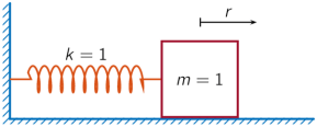
A one-dimensional discrete-time oscillating system consists of a unit mass, m, attached to a wall by a spring of unit elastic constant. A sensor samples the acceleration, a, of the mass at Fs=5 Hz.

Mass-spring system, with a mass of 1 kilogram and a spring with elastic constant k=1 Newton per meter. The displacement of the mass is r (in meters).

Generate 50 time samples. Define the sampling interval Δt=1/Fs.

Fs = 5;
dt = 1/Fs;
N = 50;
t = dt*(0:N-1);
u = [1 zeros(1,N-1)];

The transfer function of the system has an analytic expression:

H(z)=1-z-1(1+cosΔt)+z-2cosΔt1-2z-1cosΔt+z-2.

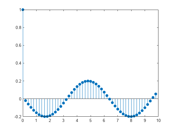
The system is excited with a unit impulse in the positive direction. Compute the time evolution of the system using the transfer function. Plot the response.

bf = [1 -(1+cos(dt)) cos(dt)];
af = [1 -2*cos(dt) 1];
yf = filter(bf,af,u);
stem(t,yf,"o")
xlabel("t")

Figure contains an axes object. The axes object with xlabel t contains an object of type stem.

Compute the time-dependent acceleration using the second-order sections representation of the transfer function to filter the input. Plot the result. The result is the same in both cases.

sos = tf2sos(bf,af);
yt = sosfilt(sos,u);
stem(t,yt,"filled")

Figure contains an axes object. The axes object contains an object of type stem.

Input Arguments

collapse all

Transfer function coefficients, specified as vectors. Express the transfer function in terms of b and a as

H(z)=B(z)A(z)=b1+b2z1++bn+1zna1+a2z1++am+1zm.

Example: b = [1 3 3 1]/6 and a = [3 0 1 0]/3 specify a third-order Butterworth filter with normalized 3 dB frequency 0.5π rad/sample.

Data Types: double

Row order, specified as one of the following:

  • 'up' — Order the sections so the first row of sos contains the poles farthest from the unit circle.

  • 'down' — Order the sections so the first row of sos contains the poles closest to the unit circle.

Data Types: char

Scaling of gain and numerator coefficients, specified as one of the following:

  • 'none' — Apply no scaling.

  • 'inf' — Apply infinity-norm scaling.

  • 'two' — Apply 2-norm scaling.

Using infinity-norm scaling with 'up'-ordering minimizes the probability of overflow in the realization. Using 2-norm scaling with 'down'-ordering minimizes the peak round-off noise.

Note

Infinity-norm and 2-norm scaling are appropriate only for direct-form II implementations.

Data Types: char

Output Arguments

collapse all

Second-order section representation, returned as a matrix. sos is an L-by-6 matrix

sos=[b01b11b211a11a21b02b12b221a12a22b0Lb1Lb2L1a1La2L]

whose rows contain the numerator and denominator coefficients bik and aik of the second-order sections of H(z):

H(z)=gk=1LHk(z)=gk=1Lb0k+b1kz1+b2kz21+a1kz1+a2kz2.

Overall system gain, returned as a real scalar.

If you call tf2sos with one output argument, the function embeds the overall system gain in the first section, H1(z), so that

H(z)=k=1LHk(z).

Note

Embedding the gain in the first section when scaling a direct-form II structure is not recommended and can result in erratic scaling. To avoid embedding the gain, use tf2sos with two outputs.

Algorithms

tf2sos uses a four-step algorithm to determine the second-order section representation for an input transfer function system:

  1. It finds the poles and zeros of the system given by b and a.

  2. It uses the function zp2sos, which first groups the zeros and poles into complex conjugate pairs using the cplxpair function. zp2sos then forms the second-order sections by matching the pole and zero pairs according to the following rules:

    1. Match the poles closest to the unit circle with the zeros closest to those poles.

    2. Match the poles next closest to the unit circle with the zeros closest to those poles.

    3. Continue until all of the poles and zeros are matched.

    tf2sos groups real poles into sections with the real poles closest to them in absolute value. The same rule holds for real zeros.

  3. It orders the sections according to the proximity of the pole pairs to the unit circle. tf2sos normally orders the sections with poles closest to the unit circle last in the cascade. You can tell tf2sos to order the sections in the reverse order by specifying order as 'down'.

  4. tf2sos scales the sections by the norm specified in scale. For arbitrary H(ω), the scaling is defined by

    Hp=[12π02π|H(ω)|pdω]1/p

    where p can be either ∞ or 2. See the references for details on the scaling. The algorithm follows this scaling in an attempt to minimize overflow or peak round-off noise in fixed-point filter implementations.

References

[1] Jackson, L. B. Digital Filters and Signal Processing. 3rd ed. Boston: Kluwer Academic Publishers, 1996.

[2] Mitra, S. K. Digital Signal Processing: A Computer-Based Approach. New York: McGraw-Hill, 1998.

[3] Vaidyanathan, P. P. “Robust Digital Filter Structures.” Handbook for Digital Signal Processing (S. K. Mitra and J. F. Kaiser, eds.). New York: John Wiley & Sons, 1993.

Extended Capabilities

Version History

Introduced before R2006a