Design PID Control for DC Motor Using Classical Control Theory

Open Model

Open the DesignDCMotorPIDControl model.

myModel = "DesignDCMotorPIDControl";
open_system(myModel);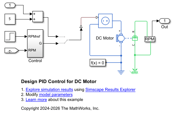

In this example, you model a DC Motor driven by a Controlled Voltage Source block. The Control block provides the control command, which is the voltage applied by the Controlled Voltage Source. You can run the system using closed-loop control or an open-loop.

First, you linearize the model, plot the frequency response, and compute the phase margin. Then, you design a proportional control, which changes the magnitude of the Bode plot but does not change the phase. This control reduces oscillations but introduces a larger steady-state error due to the lower gain. You then design a PI control, which changes both the gain and phase. This controller eliminates the steady-state error, but the response is slower. Finally, you design a PID control, which introduces a response to the derivative of the output, speeding up the response.

Linearize Averaged Switching Model and Plot Frequency Response

Set up the model to allow linearization. Set the model to start from steady state and configure the inputs to run in open loop.

set_param(myModel + "/Solver Configuration",DoDC="on");
set_param(myModel + "/Manual Switch",sw="1");

Linearize the model using the linearize (Simulink Control Design) function. Define linearization I/O points at the Manual Switch input and the PS-Simulink Converter output (angular speed) to obtain the open-loop plant transfer function as a state-space object.

io(1) = linio(myModel + "/Manual Switch",1,'input');
io(2) = linio(myModel + "/Sensing/PS-Simulink Converter",1,'output');
SS = linearize(myModel,io);

The transfer function is the Laplace transform of the impulse response of the open-loop system. This equation defines the transfer function in terms of the state-space matrices:

The variable to control is the output speed. Compute the open-loop transfer function G from the state-space representation matrices A, B, C, and D.

G = @(w) SS.C*(1i*w*eye(size(SS.A))-SS.A)^-1*SS.B + SS.D;

Plot the Bode diagram of the open-loop plant.

figure;
bp = bodeplot(SS);
grid on;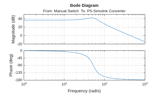 

Compute Stability Margins

To calculate the gain and phase margins, use the margin function. The phase margin is determined at the gain crossover frequency (where the gain is 0 dB), and the gain margin is determined at the phase crossover frequency (where the phase is $$-180^o$$).

[Gm,Pm,Wcg,Wcp] = margin(SS)

Gm = 
Inf

Pm = 
3.8330

Wcg = 
NaN

Wcp = 
432.9472

Plot the Bode diagram with stability margins annotated.

bp.Characteristics.MinimumStabilityMargins.Visible = 'on';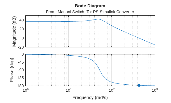

grid on;

Plot the closed-loop step response.

designDCMotorPIDControlPlotRPM("P");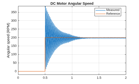

The small phase margin of the open-loop indicates the closed-loop system is very close to instability. Consequently, the step response oscillates until the response settles down. Also, a small steady-state error indicates that the control needs integral action.

Design Proportional Controller

The plant is already stable. A proportional controller could speed up the response but also make it unstable.

A proportional controller changes the magnitude of the Bode plot while the phase remains the same.

Choose a crossover frequency with a sufficient phase margin. In this case, 15 Hz allows a phase margin of around $$24^o$$, which is not yet sufficient but better than the current value.

crossoverFreqP = 15; % Hz
pulsationP = crossoverFreqP*2*pi; % rad/s
phaseMarginP = 180 + angle(G(pulsationP))/pi*180 % deg

phaseMarginP = 
23.7178

Calculate the proportional controller gain.

Kp = 1/abs(G(pulsationP))

Kp = 
0.0362

Create the proportional controller using the pid command.

C_P = pid(Kp)

C_P = 
  Kp = 0.0362
 
P-only controller.
Model Properties

Plot the Bode diagrams of the plant and the open-loop transfer function with the proportional control, including stability margins.

L_P = C_P * SS;
figure;
bodeplot(SS)
hold on;
margin(L_P); grid on;
legend("Plant","Kp * Plant");

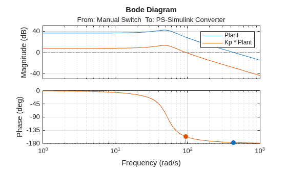
Verify that the closed-loop system is now stable by plotting the output voltage of the converter.

[num,den] = tfdata(tf(C_P),'v');
designDCMotorPIDControlPlotRPM("P")

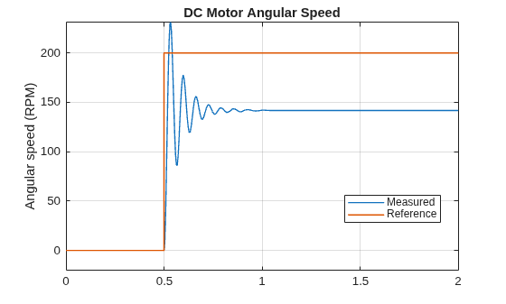
Although the oscillations are significantly reduced, the plot now shows a larger a steady-state error due to the lower gain. If you calculate and observe the closed-loop transfer function, the order of the numerator and denominator polynomials is the same, which indicates a finite error at steady state for a step input.

Design Proportional-Integral Controller

A proportional-integral controller changes both the gain and the phase of the open-loop Bode plot. The transfer function of the PI control in standard form is:

where:

This is the same structure as the pidstd standard form used by the pidtune function.

To calculate the gains analytically, use the relation of the control gain and phase. From the Bode plot, determine the control gain and phase you need, and then use this expression to calculate the gains:

where:

Firstly, determine the value of the crossover frequency and the phase margin. A reduction in speed improves the steady-state accuracy. Reduce around 10-20% of the crossover frequency.

crossoverFreqPI = 10; % Hz
phaseMarginPI = 50; % deg
pulsationPI = crossoverFreqPI*2*pi; % rad/s

Then, calculate the amplitude and phase of the plant at this frequency.

gainGpulsationPI = abs(G(pulsationPI));
gainGpulsationPIdB = 20*log10(abs(G(pulsationPI)));
angleGpulsationPI = angle(G(pulsationPI))/pi*180; % deg
controlPhase = -180 + phaseMarginPI - angleGpulsationPI % deg

controlPhase = 
-6.3275

The control has an angle of around $$-6^o.$$ Match the phases of both sides of the previous equation to obtain the value of $$T_i$$.

$$\angle \left(1+\frac{1}{T_i\omega j}\right)={\varphi }_C$$; since $$\frac{1}{T_i\omega j}=\frac{-j}{T_i\omega }$$, the phase is $$\arctan \left(\frac{-1}{T_i\omega }\right)$$

Then: $$T_i\omega =\tan (90^{\circ }+{\varphi }_C)$$

Ti = tand(controlPhase+90)/pulsationPI

Ti = 
0.1435

Calculate the gain of the plant at the gain crossover frequency and obtain the value of the proportional controller gain.

controlPIGain = 1/gainGpulsationPI;
Kp = controlPIGain / sqrt(1 + 1/(Ti*pulsationPI)^2)

Kp = 
0.0116

Alternatively, use pidtune with the desired crossover frequency and phase margin to obtain the PI controller.

opts = pidtuneOptions('PhaseMargin',phaseMarginPI);
C_PI = pidstd(1,1,0);
C_PI = pidtune(SS, C_PI, pulsationPI,opts)

C_PI = 
             1      1 
  Kp * (1 + ---- * ---)
             Ti     s 

  with Kp = 0.0116, Ti = 0.144
 
Continuous-time PI controller in standard form
Model Properties

Note that the gains are the same for both the manual method and using the pidtune function.

Plot the Bode diagrams of the plant and the open-loop transfer function with the PI controller, including stability margins.

L_PI = C_PI * SS;
figure;
bodeplot(SS);
grid on; hold on;
margin(L_PI);
legend("Plant","PI * Plant");

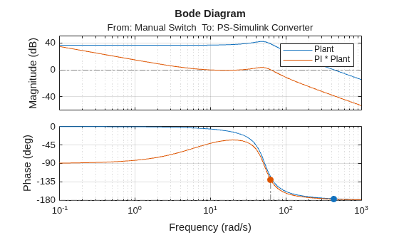
Plot the closed-loop step response.

[num,den] = tfdata(tf(C_PI),'v');
designDCMotorPIDControlPlotRPM("PI")

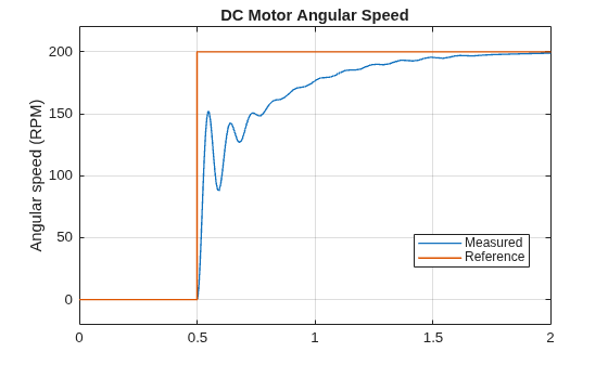
The integral control successfully eliminates the steady-state error. However, the response is now slower. You need derivative action to speed up the response.

Design Proportional-Integral-Derivative Controller

A proportional-integral-derivative controller changes both the gain and the phase of the open-loop Bode plot. The control introduces a response to the derivative of the output, which makes the controller faster. The transfer function of the PID control in standard form is:

$$C(s)=K_P\left(1+\frac{1}{T_{i}s}+\frac{T_{d}s}{\frac{T_d}{N}s+1}\right)$$,

where:

This is the same structure as the pidstd standard form used by the pidtune function.

To calculate the gains analytically, evaluate the controller at $$s=j\omega$$. The real and imaginary parts of the controller response are:

$$\frac{C(j\omega )}{K_P}=\underset{R}{\underbrace{\stackrel{}{1+\frac{(T_d\omega {)}^2/N}{1+(T_d\omega /N{)}^2}}}}+j\underset{I}{\underbrace{\stackrel{}{\left(-\frac{1}{T_i\omega }+\frac{T_d\omega }{1+(T_d\omega /N{)}^2}\right)}}}$$,

At the gain crossover frequency, $$|C(j\omega )\cdot G(j\omega )|=1$$ and the phase of the product determines the phase margin:

There are four parameters to determine ($$K_P$$, $$T_i$$, $$T_d$$, and $$N$$). After you choose the phase margin and crossover frequency, you select the integral time constant and filtering factor, then solve for the derivative time constant and proportional gain.

To start, choose the gain crossover frequency and phase margin. The derivative action compensates for the lag from the integral component, so you can select a frequency greater than the integral and proportional control. Choose a crossover frequency superior to the crossover frequency of the plant and a phase margin larger than the integral control.

crossoverFreqPID = 100; % gainCrossoverPulsation; % Hz
phaseMarginPID = 70; % deg

The control gain is the inverse of the plant at the crossover frequency.

gainGpulsationPID = abs(G(crossoverFreqPID*2*pi));
controlPIDGain = 1/gainGpulsationPID;

Calculate the control phase shift. The control phase is the difference between the plant phase and the angle given by the phase margin $$(-180^{\circ }+{\varphi }_M)$$.

pulsationPID = crossoverFreqPID*2*pi; % rad/s
angleGpulsationPID = angle(G(pulsationPID))/pi*180; % deg
controlPhase = -180 + phaseMarginPID - angleGpulsationPID; % deg

Determine the integral time constant $$T_i$$ like you did for the PI control. Choose an angle for the integral contribution and calculate $$T_i$$.

integralPhase = -15; % deg
Ti = tand(integralPhase+90)/pulsationPID

Ti = 
0.0059

Choose a value of $$N$$ for the derivative filter. A higher $$N$$ allows more derivative action but also amplifies noise.

N = 100;

With $$T_i$$ and $$N$$ fixed, solve for $$T_d$$ from the phase equation. Substituting $$x=T_d\omega /N$$ gives a quadratic equation:

$$\left[\tan ({\varphi }_C)(1+N)-a\right]x^2-Nx+\left[\tan ({\varphi }_C)-a\right]=0$$, where $$a=-\frac{1}{T_i\omega }$$

t = tand(controlPhase);
a = -1/(Ti*pulsationPID);
A_coeff = t*(1+N) - a;
B_coeff = -N;
C_coeff = t - a;
x = (-B_coeff + sqrt(B_coeff^2 - 4*A_coeff*C_coeff)) / (2*A_coeff);
Td = N*x/pulsationPID

Td = 
0.0610

Next, calculate the proportional gain using the amplitude equation derived from the control equation:

R = 1 + (Td*pulsationPID)^2/N / (1 + (Td*pulsationPID/N)^2);
I = -1/(Ti*pulsationPID) + Td*pulsationPID / (1 + (Td*pulsationPID/N)^2);
Kp = controlPIDGain / sqrt(R^2 + I^2)

Kp = 
0.0590

Alternatively, instead of all this process, use pidtune with the desired crossover frequency and phase margin to obtain the PIDF controller (PID with derivative filter).

opts = pidtuneOptions('PhaseMargin',phaseMarginPID);
C_PID_function = pidstd(1,1,1,1);
C_PID_function = pidtune(SS,C_PID_function,pulsationPID,opts)

C_PID_function = 
             1      1              s      
  Kp * (1 + ---- * --- + Td * ------------)
             Ti     s          (Td/N)*s+1 

  with Kp = 0.481, Ti = 0.0285, Td = 0.0069, N = 496
 
Continuous-time PIDF controller in standard form
Model Properties

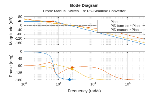
Please note that the parameters are different. This is because the pidtune function has only two design parameters, phase margin and control pulsation, and you cannot fix the filter constant $$N$$ value, resulting in different control parameters, but equally valid for the design parameters. Both use the same standard form structure.

Plot the Bode diagrams of the plant and the open-loop transfer function with the PID controller, both for the manual and pidtune function methods, including stability margins.

L_PID_function = C_PID_function * SS;
C_PID_manual = pidstd(Kp, Ti, Td, N);
L_PID_manual= ss(C_PID_manual) * SS;
figure;
bodeplot(SS);
grid on; hold on;
margin(L_PID_function);
margin(L_PID_manual);
legend("Plant","PID function * Plant", "PID manual * Plant");

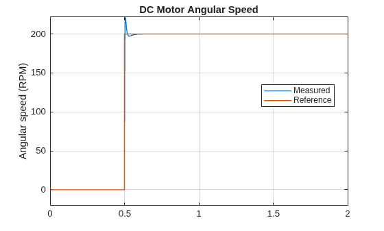
Plot the closed-loop step response.

[num,den] = tfdata(tf(C_PID_function),'v');
designDCMotorPIDControlPlotRPM("PID");

[num,den] = tfdata(tf(C_PID_manual),'v');
designDCMotorPIDControlPlotRPM("PID");

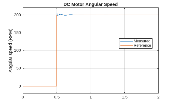
The PID controller significantly improves the response time compared to the PI controller.