Design PID Control for DC Motor Using Root Locus

R2026b

Since R2026b

This example uses:

Simulink Control Design Simulink Control Design

This example shows how to design a PID controller for a DC Motor using the root locus method. This method places the poles and the zeros strategically to obtain the closed-loop desired response. Alternatively, you can use Steady State Manager, Model Linearizer, Frequency Response Estimator, or PID tuner apps to streamline the design.

To design the controller using root locus, you need a linearized model.

Open Model

Open the DesignDCMotorPIDControl model.

myModel = "DesignDCMotorPIDControl";
open_system(myModel);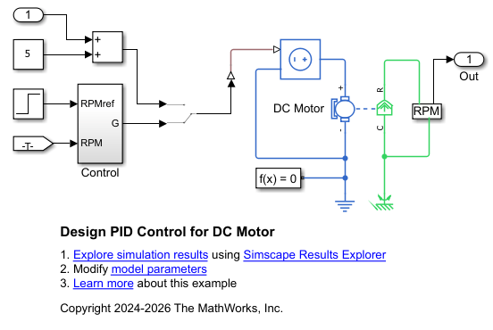

In this example, you model a DC Motor driven by a Controlled Voltage Source block. The Control block provides the control command, which is the voltage applied by the Controlled Voltage Source. You can run the system using closed-loop control or an open-loop.

First, you linearize the model, plot the frequency response, and compute the phase margin. Then, you design a proportional control, which changes the magnitude of the Bode plot but does not change the phase. This control reduces oscillations but introduces a larger steady-state error due to the lower gain. You then design a PI control, which changes both the gain and phase. This controller eliminates the steady-state error, but the response is slower. Finally, you design a PID control, which introduces a response to the derivative of the output, speeding up the response.

Linearize Averaged Switching Model and Plot Frequency Response

Set up the model to allow linearization. Set the model to start from steady state and configure the inputs to run in open loop.

set_param(myModel + "/Solver Configuration",DoDC="on");
set_param(myModel + "/Manual Switch",sw="1");

Linearize the model using the linearize (Simulink Control Design) function. Define linearization I/O points at the Manual Switch input and the PS-Simulink Converter output (angular speed) to obtain the open-loop plant transfer function as a state-space object.

io(1) = linio(myModel + "/Manual Switch",1,'input');
io(2) = linio(myModel + "/Sensing/PS-Simulink Converter",1,'output');
SS = linearize(myModel,io);

The transfer function is the Laplace transform of the impulse response of the open-loop system. This equation defines the transfer function in terms of the state-space matrices:

$G (s) = C (s I - A)^{- 1} B + D$

The variable to control is the output speed. Compute the open-loop transfer function G from the state-space representation matrices A, B, C, and D.

G = @(w) SS.C*(1i*w*eye(size(SS.A))-SS.A)^-1*SS.B + SS.D;
Gs = @(s) SS.C*(s*eye(size(SS.A))-SS.A)^-1*SS.B + SS.D;

Plot the Bode diagram of the open-loop plant.

figure;
bp = bodeplot(SS);
grid on;

To calculate the gain and phase margins, use the margin function. The phase margin is determined at the gain crossover frequency (where the gain is 0 dB), and the gain margin is determined at the phase crossover frequency (where the phase is $- 18 0^{o}$ ).

[Gm,phaseMargin,Wcg,gainCrossoverPulsation] = margin(SS)

Gm = 
Inf

phaseMargin = 
3.8330

Wcg = 
NaN

gainCrossoverPulsation = 
432.9472

Plot the Bode diagram with stability margins annotated.

bp.Characteristics.MinimumStabilityMargins.Visible = 'on';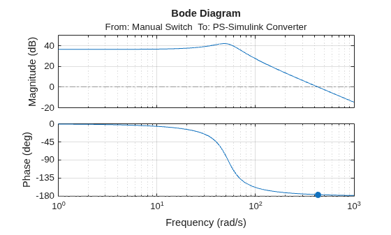

MATLAB figure

grid on;

Visualize the poles and zeros:

Gtf = tf(SS);

Plot the root locus of the open loop.

figure; pzplot(Gtf);
xlim([-30, 10]);
ylim([-100 100]);

MATLAB figure

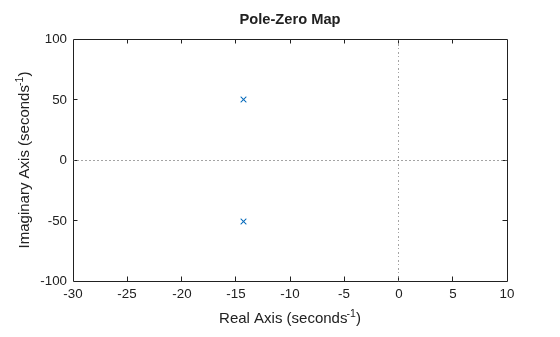
poles = pole(Gtf)

poles = 2×1 complex

 -14.2905 +50.4700i
 -14.2905 -50.4700i

zeros = zero(Gtf)

zeros = 
-5.8824e+09

The poles have small negative real parts, indicating the system is stable. The poles form a complex conjugate pair, so the system is underdamped but not oscillatory. The zero lies several orders of magnitude further left, making its effect negligible.

Plot the open-loop step response.

designDCMotorPIDControlPlotRPM("P");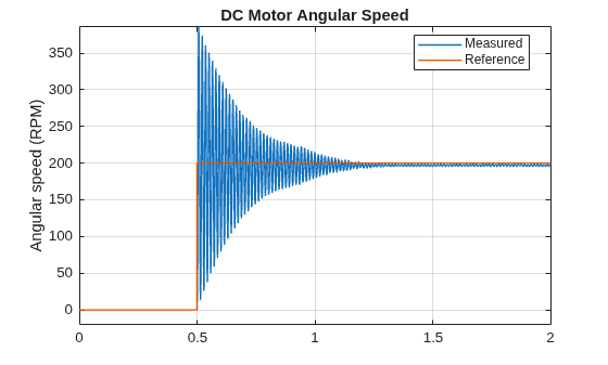

Figure contains an axes object. The axes object with title DC Motor Angular Speed, ylabel Angular speed (RPM) contains 2 objects of type line. These objects represent Measured, Reference.

The overshoot is almost 90% and the settling time is more than a second. This corroborates the information obtained from the poles, which is that this is an underdamped, but stable system. The steady-state error is very small.

Design Proportional Controller

The plant is already stable. A proportional controller could speed up the response, but also increase the steady state error.

In order to design a proportional controller, choose some response specifications to meet. To calculate the gain of the proportional control, there is only one degree of freedom, which means you can only meet one requirement. In this case, you aim to reduce the overshoot down to 65%. If you reduce it more, the steady-state error might increase too much in this case. A specific overshoot translates in the complex chart as a line that starts at the origin and extend to the negative part of the plane with an angle equal to $θ$ , obtained from the following expression:

$M_{p} = e^{\frac{π}{\tan θ}}$

Mp.P = 0.65;
theta.P = atand(-pi/log(Mp.P));

Calculate the real and negative components of the roots of the closed-loop system. The real component is the same as the open-loop poles because the proportional control changes only the gain, and not the phase of the system. The new roots of the closed-loop system are therefore in the root locus of the plant.

RootReal.P = real(poles(1));

As for the imaginary component, calculate the intersection of the root locus with the damping contour.

RootImaginary.P = RootReal.P*tand(theta.P);

The roots of the closed-loop system that meet the requirement are:

S.P1 = RootReal.P - RootImaginary.P*j;
S.P2 = RootReal.P + RootImaginary.P*j;
figure; rlocus(Gtf); 
control = "P"; DesignPIDControlForDCMotorUsingRootLocusPlotRoots;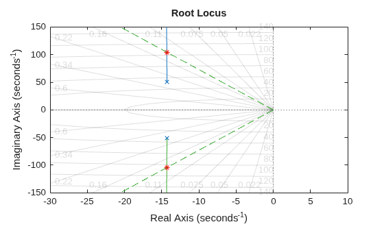

MATLAB figure

You now apply the module criterion to obtain the proportional controller gain of the system with those dominant poles.

$1 = | K_{p} \cdot G (s) |$

K.P = 1/abs(Gs(S.P1))

K = struct with fields:
    P: 0.0449

Plot the step response and the Bode plots.

num = [K.P]; den = [1];
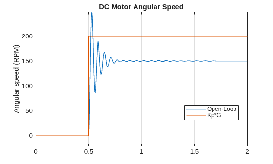
figure; designDCMotorPIDControlPlotRPM("P");
legend(["Open-Loop", "Kp*G"]);

Figure contains an axes object. The axes object with title DC Motor Angular Speed, ylabel Angular speed (RPM) contains 2 objects of type line. These objects represent Open-Loop, Kp*G.

L_P = K.P * SS;
figure; bodeplot(SS);
hold on; margin(L_P); grid on;
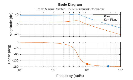
legend("Plant","Kp * Plant");

MATLAB figure

The step response now has less overshoot but is slower and has a larger steady-state error.

The Bode plot shows that the system with a proportional control has the same phase, but a smaller magnitude. This occurs because the proportional gain is less than 1. The new system also has a bigger phase margin, meaning the system is more stable. However, the crossover frequency is 1/4 of the open loop system, which indicates that the response is slower.

To reduce steady-state error and increase the speed of the system, you can add a derivative action.

Proportional Derivative Controller

The transfer function is:

$R (s) = K \frac{s + b}{s + N \cdot b}$

Adding derivative action means adding a zero and a filtering pole to the open-loop transfer function. This moves the roots to the left, which increases the speed of the dominant poles. You can choose a faster frequency for the roots of the system. In this case, choose a speed twice as fast as the roots of the system with proportional control:

wn.PD = 2*abs(S.P1)

wn = struct with fields:
    PD: 210.3839

Now choose a value for the overshoot that is smaller than the previous ones so the system will be faster.

Overshoot $M_{p}$ < 15%

$\begin{array}{l} M_{p} < 0.15; \\ M_{p} = e^{\frac{π}{\tan θ}} \\ ζ = \cos θ; \end{array}$

$θ \leq \arctan (- p i / l o g (0.15)) = 5 8^{o}$

Mp.PD = 0.3;
theta.PD = atand(-pi/log(Mp.PD))

theta = struct with fields:
     P: 82.1922
    PD: 69.0313

zeta = cosd(theta.PD); % damping ratio
RootReal.PD = -wn.PD*zeta;
RootImaginary.PD = wn.PD*sind(theta.PD);

The points $S_{*}$ chosen are inside the area, but with a higher gain to obtain a smaller steady-state error.

S.PD1 = RootReal.PD + RootImaginary.PD*j;
S.PD2 = RootReal.PD - RootImaginary.PD*j;

Using the criteria of the argument, introduce a zero $b$ and a filtering pole $N \cdot b$ so that the branches of the rlocus go through the chosen points. Calculate the angle $ϕ$ that the zero must add.

$ϕ = - 18 0^{o} + α_{1} + α_{2} + α 3$

where:

$α_{1}$ is the angle between the new roots and the first plant pole.
$α_{2}$ is the angle between the new roots and the second plant pole.
$α_{2}$ is the angle between the new roots and the new pole $N \cdot b$ .

The new pole must have a high pulsation where it does not act as a dominant one, but filters high frequencies. To ease the calculations, assume that the new pole has no imaginary part.

Nb = 2*pi*1000;
phi.PD = (-pi + angle(S.PD1-poles(1)) + angle(S.PD1-poles(2)) + angle(S.PD1+Nb) - angle(S.PD1-zeros))/pi*180;
b.PD = abs(-real(S.PD1) + imag(S.PD1)/tand(phi.PD));
figure; rlocus(Gtf, linspace(0, 2, 1000));
control = "PD"; DesignPIDControlForDCMotorUsingRootLocusPlotRoots;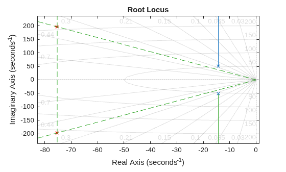

MATLAB figure

By the criteria of the module, obtain K:

$1 = | K \frac{(s + b)}{(s + N b)} \cdot G (s) |$

K.PD = abs(S.PD1+Nb)/abs(Gs(S.PD1)*(S.PD1+b.PD))

K = struct with fields:
     P: 0.0449
    PD: 4.2661

Plot the new root locus of the system with the derivative action to verify that the chosen roots are overlayed.

Control.PD = tf(K.PD*[1 b.PD], [1 Nb]);
H.PD = feedback(Gtf*Control.PD, 1);
figure; rlocus(Gtf*Control.PD, linspace(0, 2, 1000)); 
control = "PD"; DesignPIDControlForDCMotorUsingRootLocusPlotRoots;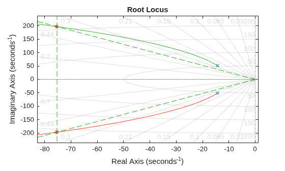

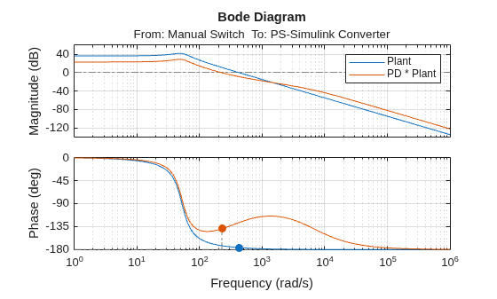
MATLAB figure

Plot the Bode plot and the step response.

L_PD = Control.PD * SS;
figure;
bodeplot(SS);
hold on;
margin(L_PD); grid on;
legend("Plant","PD * Plant");

MATLAB figure

num = K.PD*[1 b.PD];
den = [1 Nb];
figure; designDCMotorPIDControlPlotRPM("PD");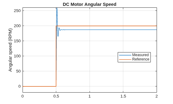

Figure contains an axes object. The axes object with title DC Motor Angular Speed, ylabel Angular speed (RPM) contains 2 objects of type line. These objects represent Measured, Reference.

The response is now much faster than that of the proportional control. The Bode plot shows that the cut-off frequency is twice that of the proportional control. However, the derivative action does not remove the steady-state error. You need integral action for that.

Proportional Integral Controller

The transfer function for a PI controller is:

$R (s) = K \frac{(s + a)}{s}$

This means adding an integrator and a zero to the transfer function. Adding an integrator cancels the steady-state error. However, the system is slower because of the integrator and the zero, which are typically at a frequency smaller than the dominant poles.

There are two parameters to obtain, $K$ and $a$ . This means you need to make two decisions to set them, in this case, you choose the overshoot and the speed of the closed-loop system roots.

You choose an overshoot $M_{p}$ to be less or equal than 55%, and calculate the lines in the complex plane where the new roots are placed.

Mp.PI = 0.6;
theta.PI = atand(-pi/log(Mp.PI));

The integral component makes the system slower, so the roots of the closed-loop system must be placed at the right of the poles in the complex plane. With the same overshoot, the pulsation is smaller than the crossover pulsation of the proportional control. In this case, you choose an even smaller overshoot, so the pulsation needs to be smaller.

wn.PI =9*2*pi; %[rad/s]

You know the distance to the origin $w_{n}$ in the complex plane and the angle from the real axis $M_{p}$ , so you can calculate the real and negative components of the roots of the system.

zeta = cosd(theta.PI);
RootReal.PI = -wn.PI*zeta;
RootImaginary.PI = wn.PI*sind(theta.PI);

The roots of the closed-loop system that meet the requirements are:

S.PI1 = RootReal.PI + RootImaginary.PI*j;
S.PI2 = RootReal.PI - RootImaginary.PI*j;

Now calculate the zero location that places the chosen roots in the root locus of the system with the proportional control.

Using the criteria of the argument, you introduce a zero so that the branches of the root locus go through the chosen points. Calculate the angle $ϕ$ that the zero must add.

$ϕ = - 18 0^{o} + α_{1} + α_{2} + α 3$

where:

$α_{1}$ is the angle between the new roots and the first plant pole.
$α_{2}$ is the angle between the new roots and the second plant pole.
$α_{3}$ is the angle between the new roots and the integrator introduced by the integral control.

phi.PI = abs(-pi + angle(S.PI1-poles(1)) + angle(S.PI1-poles(2)) +angle(S.PI1))/pi*180;

Calculate the location of the zero.

a.PI =  -(real(S.PI1) - imag(S.PI1)/tand(phi.PI))

a = struct with fields:
    PI: 52.4702

Plot the location of the new roots.

figure; rlocus(Gtf, linspace(0, 2, 1000)); 
control = "PI"; DesignPIDControlForDCMotorUsingRootLocusPlotRoots;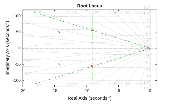

MATLAB figure

Note that the location of the roots is to the right of the system roots. This means the pulsation is smaller, as you specified before.

By the criteria of the module, obtain K:

$1 = | K \frac{s + a}{s} \cdot G (s) |$

K.PI = abs(S.PI1/(S.PI1+a.PI)/Gs(S.PI1));

Plot the new root locus of the system with the integral action to verify that the chosen roots are overlayed.

Control.PI = tf(K.PI*[1 a.PI],[1 0]);
H.PI = feedback(Gtf*Control.PI, 1);
figure; rlocus(Gtf*Control.PI, linspace(0, 5, 2000)); 
control = "PI"; DesignPIDControlForDCMotorUsingRootLocusPlotRoots;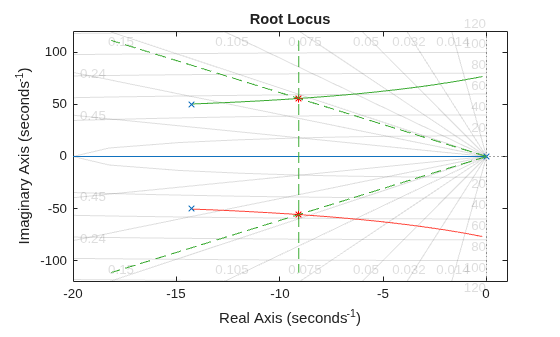

MATLAB figure

C_PI = pidstd(1,1,0);
C_PI = pidtune(SS, C_PI, wn.PI)

C_PI = 
             1      1 
  Kp * (1 + ---- * ---)
             Ti     s 

  with Kp = 0.00877, Ti = 0.0681
 
Continuous-time PI controller in standard form
Model Properties

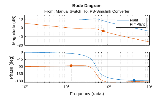
Plot the Bode plot and step response.

L_PI = Control.PI * SS;
figure;
bodeplot(SS);
hold on;
margin(L_PI); grid on;
legend("Plant","PI * Plant");

MATLAB figure

num = K.PI*[1 a.PI];
den = [1 0];
figure; designDCMotorPIDControlPlotRPM("PI");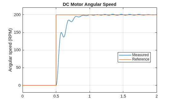

Figure contains an axes object. The axes object with title DC Motor Angular Speed, ylabel Angular speed (RPM) contains 2 objects of type line. These objects represent Measured, Reference.

The integral control successfully eliminates the steady-state error. However, the response is now slower, which is reflected in the low cut off frequency in the Bode plot. You need derivative action to speed up the response.

Proportional Derivative Integral Controller

$R (s) = K \frac{(s + a) (s + b)}{s (s + N \cdot b)}$

A PID controller adds both derivative and the integral action. The aim is to improve the transitory regime of the time response. You add an integrator, a pole, and two zeros, which combined allow you to place the roots of the system in a location in the complex plane where the response is much faster and with a smaller overshoot.

There are four parameters to obtain, $K$ , $b$ , $N$ and $a$ . This means you need to make two decisions to set them, in this case, you choose the overshoot and the speed of the closed-loop system roots.

Overshoot $M_{p}$ < 5%

$\begin{array}{l} M_{p} < 0.05; \\ M_{p} = e^{\frac{π}{\tan θ}} \\ ζ = \cos θ; \end{array}$

$θ \leq \arctan (- p i / l o g (0.15)) = 5 8^{o}$

wn.PID = 120*2*pi;
Mp.PID = 0.05;
theta.PID = atand(-pi/log(Mp.PID));
zeta = cosd(theta.PID); % damping ratio
RootReal.PID = -wn.PID*zeta;
RootImaginary.PID = wn.PID*sind(theta.PID);

The points $S_{*}$ chosen are inside the area, but with a higher gain to obtain a smaller steady-state error.

S.PID1 = RootReal.PID + RootImaginary.PID*j;
S.PID2 = RootReal.PID - RootImaginary.PID*j;

The plant dominant poles have a natural frequency of around 50 rad/s. Choose a pulsation for the control zeros half that of the plant poles so the dominant poles remain properly shaped by feedback. Locating the zeros below the dominant poles allows the controller to improve the damping and transient response by compensating for the part of the phase lag introduced by the complex poles. The separation between the zeros and poles preserves robustness to modeling uncertainty and parameter variations. Overall, this choice results in a well‑damped closed‑loop response while maintaining a clear and robust loop‑shaping structure.

a.PID = abs(poles(1))/2;
b.PID = abs(poles(2))/2;

Plot the location of the new roots.

figure; rlocus(Gtf, linspace(0, 2, 1000)); 
control = "PID"; DesignPIDControlForDCMotorUsingRootLocusPlotRoots;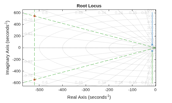

MATLAB figure

The roots are to the left of the system roots and in an area with a smaller overshoot. This positioning results in a faster system with less overshoot. The integral action eliminates steady-state error.

Using the criteria of the argument, you introduce a zero so that the branches of the root locus go through the chosen points. Calculate the angle $ϕ$ that the zero must add.

$ϕ = - 18 0^{o} + α_{p 1} + α_{p 2} + α_{s} - α_{z}$

where:

$α_{p 1}$ is the angle between the new roots and the first plant pole.
$α_{p 2}$ is the angle between the new roots and the second plant pole.
$α_{s}$ is the angle between the new roots and the integrator introduced by the integral control.
$α_{z}$ is the angle between the new roots and the integral controller's zero.

phi.PID = -(-pi + angle(S.PID1-poles(1)) + angle(S.PID1-poles(2)) + angle(S.PID1) - angle(S.PID1-(-a.PID))- angle(S.PID1-(-b.PID)))/pi*180;
N.PID = 1/abs(b.PID)*(imag(S.PID1)/tand(phi.PID)-real(S.PID1));

By the criteria of the module, obtain K:

$1 = | K_{P I D} \cdot \frac{(s + a) (s + b)}{s \cdot (s + N \cdot b)} \cdot G (s) |$

K.PID = abs(1/Gs(S.PID1)...
    *S.PID1/(S.PID1+a.PID)/(S.PID1+b.PID)*(S.PID1+abs(b.PID)*N.PID));

Plot the new root locus of the system with the derivative action to verify that the chosen roots are overlayed.

Control.PID = tf(K.PID*[1 b.PID+a.PID b.PID*a.PID],[1 abs(b.PID)*N.PID 0]);
figure; rlocus(Gtf*Control.PID, linspace(0, 2, 1000));
control = "PID"; DesignPIDControlForDCMotorUsingRootLocusPlotRoots;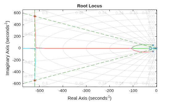

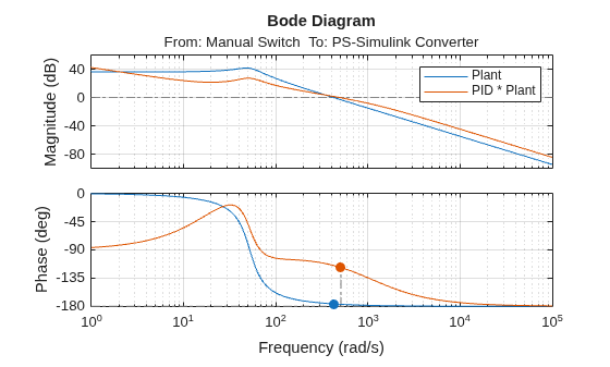
MATLAB figure

L_PID = Control.PID * SS;
figure;
bodeplot(SS);
hold on;
margin(L_PID); grid on;
legend("Plant","PID * Plant");

MATLAB figure

num = K.PID*[1 b.PID+a.PID b.PID*a.PID];
den = [1 abs(b.PID)*N.PID 0];
figure; designDCMotorPIDControlPlotRPM("PID");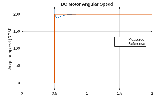

Figure contains an axes object. The axes object with title DC Motor Angular Speed, ylabel Angular speed (RPM) contains 2 objects of type line. These objects represent Measured, Reference.

Design PID Control for DC Motor Using Root Locus

Open Model

Linearize Averaged Switching Model and Plot Frequency Response

Design Proportional Controller

Proportional Derivative Controller

Proportional Integral Controller

Proportional Derivative Integral Controller

See Also

Simscape Blocks

Functions

Topics