Frequency Response Estimation to Measure Input Admittance and Output Impedance of Boost Converter

Boost Converter Model

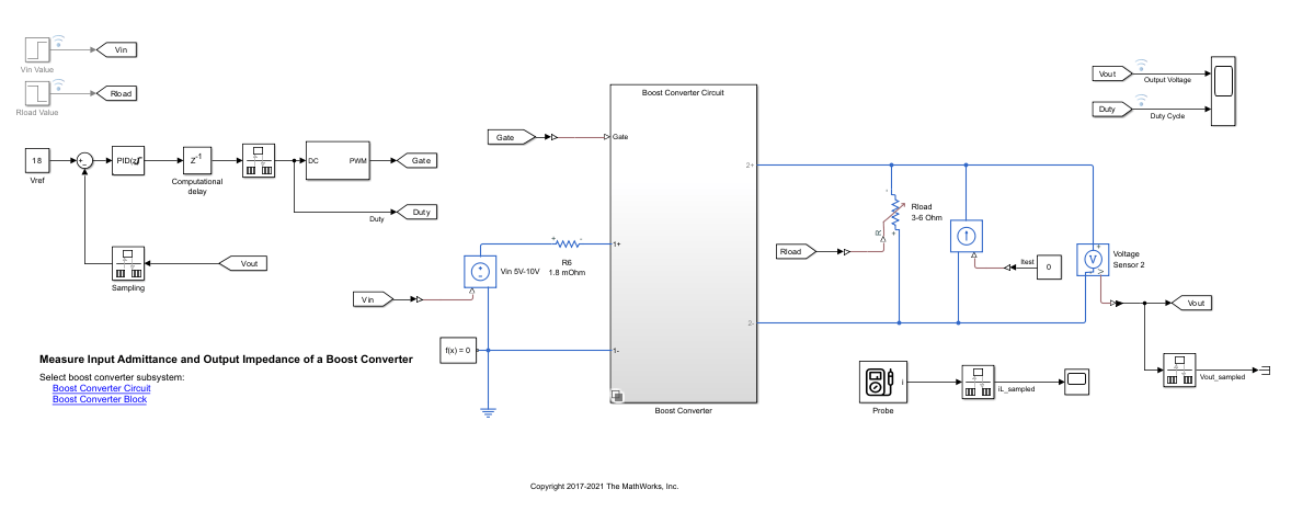
This example uses a model based on the boost converter model scdboostconverter. The original model is modified for these measurements as follows.

You can examine this model for more details.

Open the model.

mdl = 'scdboostconverterMeasureAdmittanceImpedance';
open_system(mdl)

To use the Boost Converter block version of the subsystem, in the model, click Boost Converter Block or use the following command.

set_param([mdl '/Boost Converter'],...
    'OverrideUsingVariant','block_boost_converter')

Create Pseudorandom Binary and Sinestream Input Signals for Estimation

A pseudorandom binary signal (PRBS) is a periodic, deterministic signal with white-noise-like properties that shifts between two values. A PRBS is an inherently periodic signal with a maximum period length of $2^{\mathit{n}}-1$, where $\mathit{n}$ is the PRBS order. For more information, see PRBS Input Signals.

Create a PRBS with the following configuration:

in_PRBS = frest.PRBS('Order',14,'NumPeriods',1,'Amplitude',1,'Ts',5e-6);

Create a sinestream input signal with 30 frequencies between 200 rad/s and 600,000 rad/s. Set the amplitude of the input signal to 0.5 to make it consistent with the PRBS input signal.

in_Sinestream = frest.createFixedTsSinestream(5e-06,{200,6e5});
in_Sinestream.Amplitude = 0.5;

Using different input signals leads to a different simulation time for the frequency response estimation process. To achieve similar results, the PRBS input signal typically takes a much shorter simulation time than the sinestream input signal. Here, in_PRBS takes about 15% of the simulation time as in_Sinestream.

Display the simulation time for frequency response estimation by in_PRBS.

in_PRBS.getSimulationTime

ans = 
0.0819

Display the simulation time for frequency response estimation by in_Sinestream.

in_Sinestream.getSimulationTime

ans = 
0.5207

In this example, you can use these input signals to estimate frequency response models for both input admittance and output impedance measurements.

Find Model Operating Point

To estimate the frequency response for the boost converter, you must first determine the steady-state operating point at which you want the converter to operate. For more information on finding operating points, see Find Steady-State Operating Points for Simscape Models. For this example, use an operating point estimated from a simulation snapshot at 0.045 seconds.

opini = findop(mdl,0.045);

Initialize the model with the computed operating point.

set_param(mdl,'LoadInitialState','on','InitialState','getstatestruct(opini)')

Measure Input Admittance

To collect frequency response data, you can estimate the plant frequency response at the command line. To do so, first get the input and output linear analysis points from the model.

io_Yin(1) = linio([mdl,'/PID Controller'],1,'loopbreak');
io_Yin(2) = linio([mdl,'/Sampling'],1,'loopbreak');
io_Yin(3) = linio([mdl,'/Vin Value'],1,'input');
io_Yin(4) = linio([mdl,'/Rate Transition1'],1,'output');

Specify the operating point using the model initial conditions.

op_Yin = operpoint(mdl);

Find all source blocks in the signal paths of the linearization outputs that generate time-varying signals. Such time-varying signals can interfere with the signal at the linearization output points and produce inaccurate estimation results.

srcblksYin = frest.findSources(mdl,io_Yin);

To disable the time-varying source blocks, create an frestimateOptions option set and specify the BlocksToHoldConstant option.

optsYin = frestimateOptions;
optsYin.BlocksToHoldConstant = srcblksYin;

Estimate the frequency response using the PRBS input signal.

sysestYin_prbs = frestimate(mdl,io_Yin,op_Yin,in_PRBS,optsYin);

Frequency response estimation with a PRBS input signal produces results with many frequency points. Simulink Control Design software lets you estimate plant frequency response using the Model Linearizer app. You can also use Model Linearizer to further improve a frequency response estimated at the command line.

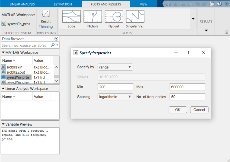
You can use Result Thinning in Model Linearizer to extract an interpolated result from an estimated frequency response model across a specified frequency range and number of frequency points. For more information, see Result Thinning.

Apply thinning to sysestYin_prbs over frequencies between 200 rad/s and 600,000 rad/s with 50 logarithmically spaced frequency points.

Click OK. The thinned model, sysestYin_prbs_thinned, appears in the MATLAB® Workspace. Alternatively, use the thinned result provided with this example.

For comparison purposes, estimate the frequency response using the defined sinestream input signal. To estimate the frequency response, run the following at the Command Window.

sysestYin_sine = frestimate(mdl,io_Yin,op_Yin,in_Sinestream,optsYin);

Because estimation with sinestream signals takes a long time, a model estimated using this input signal is provided with this example.

Measure Output Impedance

To estimate the frequency response for this model, you can use the workflow described in the previous section of this example, with slightly different settings of linear analysis points.

Get linear analysis points from the model.

io_Zout(1) = linio([mdl,'/PID Controller'],1,'loopbreak');
io_Zout(2) = linio([mdl,'/Sampling'],1,'loopbreak');
io_Zout(3) = linio([mdl,'/Constant'],1,'input');
io_Zout(4) = linio([mdl,'/Rate Transition2'],1,'output');

Specify the operating point using the model initial conditions.

op_Zout = operpoint(mdl);

Find and disable time-varying source blocks.

srcblksZout = frest.findSources(mdl,io_Zout);
optsZout = frestimateOptions;
optsZout.BlocksToHoldConstant = srcblksZout;

Estimate the frequency response using the PRBS input signal.

sysestZout_prbs = frestimate(mdl,io_Zout,op_Zout,in_PRBS,optsZout);

Using Model Linearizer, apply Result Thinning to sysestZout_prbs over frequencies between 200 rad/s and 600,000 rad/s with 50 logarithmically spaced frequency points. Alternatively, use the thinned result provided with this example.

For comparison purposes, estimate the frequency response using the defined sinestream input signal. To estimate the frequency response, run the following at the Command Window.

sysestZout_sine = frestimate(mdl,io_Zout,op_Zout,in_Sinestream,optsZout);

Because estimation with sinestream signals takes a long time, a model estimated using this input signal is provided with this example.

Analytical Transfer Functions

Compare the estimation results to the analytical transfer functions based on component parameters. Use the following parameters from the model.

L = 20e-6;
C = 1480e-6;
R = 6;
rC = 8e-3;
rL = 1.8e-3;

To compute the analytical transfer function, you require the actual duty cycle value. For this boost converter, use the logged duty cycle at the operating point.

D = 0.734785;
d = 1-D;

Define the analytical transfer functions for input admittance and output impedance, which are based on [1], using the component parameters in the boost converter model.

Yin = tf([C*(R+rC) 1], [L*C*(R+rC) L+C*rL*(R+rC)+C*R*rC-R*D*C*rC R+rL-R*D-R^2*D*d/(R+rC)]);
Zout = tf(R*[C*rC*L L+C*rC*(rL+R*D*rC*d/(R+rC)) rL+R*D*rC*d/(R+rC)], ...
    [L*C*(R+rC) L+C*rL*(R+rC)+C*R*rC-R*D*C*rC R+rL-R*D-R^2*D*d/(R+rC)]);

For a more accurate description, account for the delay due to PWM signal in the transfer function Yin.

N = 0.5;
Ts = 5e-6;
iodelay = N*Ts; % 0.5 PWM
Yin.IODelay = iodelay;

Compare Frequency Response Data to Analytical Transfer Function

Compare frequency response estimation (FRE) results using PRBS and sinestream input signals to the analytical transfer functions over the frequency range of interest.

Load the thinned PRBS results and sinestream results from a previously saved session.

load sysest_prbs_thinned_yin_zout
load sysest_sine_yin_zout

Compare input admittance results.

figure
bode(sysestYin_prbs_thinned,'b-')
hold on
bode(sysestYin_sine,'k*-')
bode(Yin,'r--',{10,1e6})
legend('FRE result using PRBS','FRE result using sinestream','Analytical result',...
    'Location','best')
title('Input Admittance')
grid on

Compare output impedance results.

figure
bode(sysestZout_prbs_thinned,'b-')
hold on
bode(sysestZout_sine,'k*-')
bode(Zout,'r--',{10,1e6})
legend('FRE result using PRBS','FRE result using sinestream','Analytical result',...
    'Location','best')
title('Output Impedance')
grid on

Examine the Bode plots. The FRE results obtained using the PRBS input signal capture interesting frequency-domain properties. For example, around the magnitude peak, the estimated frequency response result with the PRBS input signal matches the analytical transfer function much better than the frequency response estimation result with the sinestream input signal.

Close the model.

close_system(mdl,0);

References

[1] Ahmadi, Reza, and Mehdi Ferdowsi. “Modeling Closed-Loop Input and Output Impedances of DC-DC Power Converters Operating inside Dc Distribution Systems.” In 2014 IEEE Applied Power Electronics Conference and Exposition - APEC 2014, 1131–38, 2014. https://doi.org/10.1109/APEC.2014.6803449.