Train RL Agent for Adaptive Cruise Control with Constraint Enforcement

Overview

In this example, the goal is to make an ego car travel at a set velocity while maintaining a safe distance from a lead car by controlling longitudinal acceleration and braking. This example uses the same vehicle models and parameters as the Train DDPG Agent for Adaptive Cruise Control (Reinforcement Learning Toolbox) example.

Set the random seed and configure model parameters.

% Set random seed.
rng('default')

% Parameters
x0_lead = 50;   % Initial position for lead car (m)
v0_lead = 25;   % Initial velocity for lead car (m/s)
x0_ego = 10;    % Initial position for ego car (m)
v0_ego = 20;    % Initial velocity for ego car (m/s)
D_default = 10; % Default spacing (m)
t_gap = 1.4;    % Time gap (s)
v_set = 30;     % Driver-set velocity (m/s)
amin_ego = -3;  % Minimum acceleration for driver comfort (m/s^2)
amax_ego = 2;   % Maximum acceleration for driver comfort (m/s^2)
Ts = 0.1;       % Sample time (s)     
Tf = 60;        % Duration (s)

Learn Constraint Equation

For the ACC application, the safety signals are the ego car velocity $\mathit{v}$ and relative distance $\mathit{d}$ between the ego car and lead car. In this example, the constraints for these signals are $10\le \mathit{v}\le 30.5$ and $\mathit{d}\ge 5$. The constraints depend on the following states in $\mathit{x}$: ego car actual acceleration, ego car velocity, relative distance, and lead car velocity.

The action $\mathit{u}$ is the ego car acceleration command. The following equation describes the safety signals in terms of the action and states.

The Constraint Enforcement block accepts constraints of the form ${\mathit{f}}_{\mathit{x}}+{\mathit{g}}_{\mathit{x}}\mathit{u}\le \mathit{c}$. For this example, the coefficients of this constraint function are as follows.

To learn the unknown functions ${\mathit{f}}_{\mathit{i}}$ and ${\mathit{g}}_{\mathit{i}}$, you must first collect training data from the environment. To do so, first create an RL environment using the rlLearnConstraintACC model.

mdl = 'rlLearnConstraintACC';
open_system(mdl)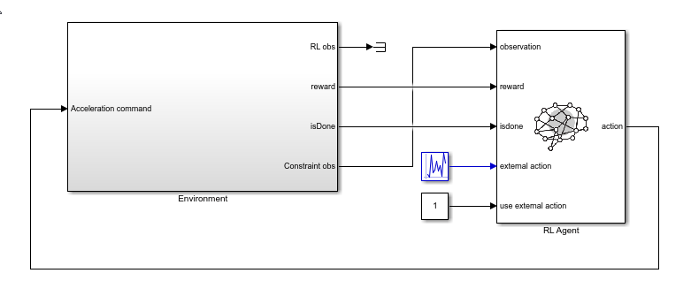

In this model, the RL Agent block does not generate actions. Instead, it is configured to pass a random external action to the environment. The purpose for using a data-collection model with an inactive RL Agent block is to ensure that the environment model, action and observation signal configurations, and model reset function used during data collection match those used during subsequent agent training.

The random external action signal is uniformly distributed in the range [10, 6]; that is, the ego car has a maximum braking power of -10 m/s^2 and a maximum acceleration power of 6 m/s^2.

For training, the four observations from the environment are the relative distance between the vehicles, the velocities of the lead and ego cars, and the ego car acceleration. Define a continuous observation space for these values.

obsInfo = rlNumericSpec([4 1]);

The action output by the agent is the acceleration command. Create a corresponding continuous action space with acceleration limits.

actInfo = rlNumericSpec([1 1],'LowerLimit',-3,'UpperLimit',2);

Create an RL environment for this model. Specify a reset function to set a random position for the lead car at the start of each training episode or simulation.

agentblk = [mdl '/RL Agent'];
env = rlSimulinkEnv(mdl,agentblk,obsInfo,actInfo);
env.ResetFcn = @(in)localResetFcn(in);

Next, create a DDPG reinforcement learning agent, which supports continuous actions and observations, using the createDDPGAgentBACC helper function. This function creates critic and actor representations based on the action and observation specifications and uses the representations to create a DDPG agent.

agent = createDDPGAgentACC(Ts,obsInfo,actInfo);

To collect data, use the collectDataACC helper function. This function simulates the environment and agent and collects the resulting input and output data. The resulting training data has nine columns.

For this example, load precollected training data. To collect the data yourself, set collectData to true.

collectData = false;
if collectData
    count = 1000;
    data = collectDataACC(env,agent,count);
else
    load trainingDataACC data
end

For this example, the dynamics of the ego car and lead car are linear. Therefore, you can find a least-squares solution for the safety-signal constraints; that is, $\mathit{v}={\mathit{R}}_{\mathit{v}}\mathit{I}$ and $\mathit{d}={\mathit{R}}_{\mathit{d}}\mathit{I}$, where $\mathit{I}$ is $\left[{\mathit{x}}_{\mathit{k}};{\mathit{u}}_{\mathit{k}}\right]$.

% Extract state and input data.
I = data(1:1000,[4,3,1,2,5]);
% Extract data for the relative distance in the next time step.
d = data(1:1000,6);
% Compute the relation from the state and input to relative distance.
Rd = I\d;
% Extract data for actual ego car velocity.
v = data(1:1000,8);
% Compute the relation from the state and input to ego car velocity.
Rv = I\v;

Validate the learned constraints using the validateConstraintACC helper function. This function processes the input training data using the learned constraints. It then compares the network output with the training output and computes the root mean squared error (RMSE).

validateConstraintACC(data,Rd,Rv)

Test Data RMSE for Relative Distance  = 8.118162e-04
Test Data RMSE for Ego Velocity = 1.066544e-14

The small RMSE values indicate successful constraint learning.

Train Agent with Constraint Enforcement

To train the agent with constraint enforcement, use the rlACCwithConstraint model. This model constrains the acceleration command from the agent before applying it to the environment.

mdl = 'rlACCwithConstraint';
open_system(mdl)

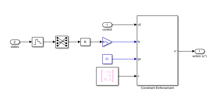
To view the constraint implementation, open the Constraint subsystem. Here, the model generates the values of ${\mathit{f}}_{\mathit{i}}$ and ${\mathit{g}}_{\mathit{i}}$ from the linear constraint relations. The model sends these values along with the constraint bounds to the Constraint Enforcement block.

Create an RL environment using this model. The action specification is the same as for the constraint-learning environment. For training, the environment produces three observations: the integral of the velocity error, the velocity error, and the ego-car velocity.

The Environment subsystem generates an isDone signal when critical constraints are violated—either the ego car has negative velocity (moves backwards) or the relative distance is less than zero (ego car collides with lead car). The RL Agent block uses this signal to terminate training episodes early.

obsInfo = rlNumericSpec([3 1]);
agentblk = [mdl '/RL Agent'];
env = rlSimulinkEnv(mdl,agentblk,obsInfo,actInfo);
env.ResetFcn = @(in)localResetFcn(in);

Since the observation specification are different for training, you must also create a new DDPG agent.

agent = createDDPGAgentACC(Ts,obsInfo,actInfo);

Specify options for training the agent. Train the agent for at most 5000 episodes. Stop training if the episode reward exceeds 260.

maxepisodes = 5000;
maxsteps = ceil(Tf/Ts);
trainingOpts = rlTrainingOptions(...
    'MaxEpisodes',maxepisodes,...
    'MaxStepsPerEpisode',maxsteps,...
    'Verbose',false,...
    'Plots','training-progress',...
    'StopTrainingCriteria','EpisodeReward',...
    'StopTrainingValue',260);

Train the agent. Training is a time-consuming process, so for this example, load a pretrained agent. To train the agent yourself instead, set trainAgent to true.

trainAgent = false;
if trainAgent
    trainingStats = train(agent,env,trainingOpts);
else
    load rlAgentConstraintACC agent
end

The following figure shows the training results.

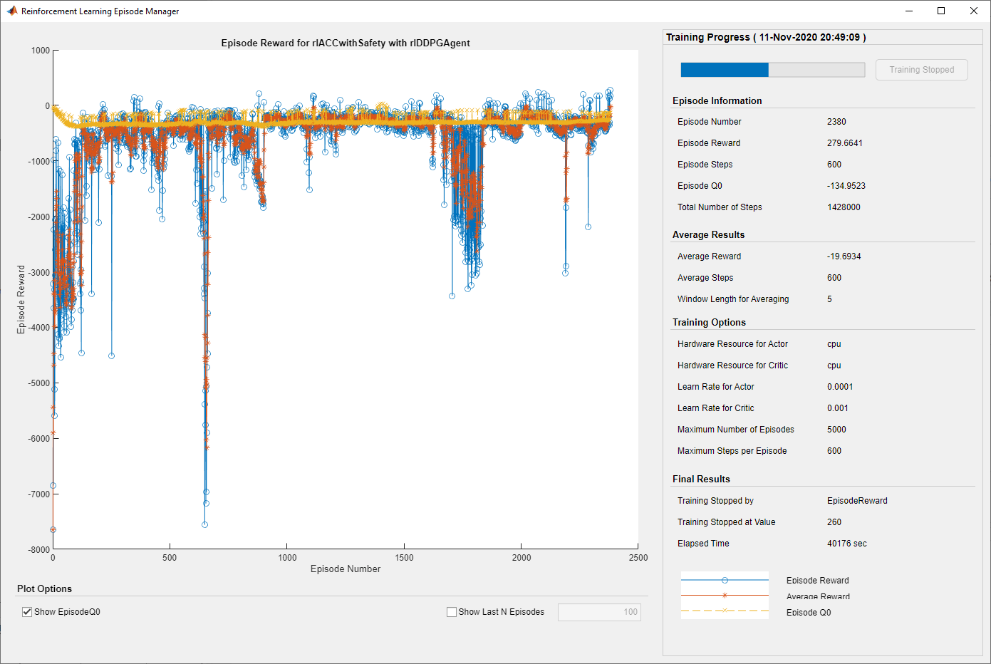
Since Total Number of Steps equals the product of Episode Number and Episode Steps, each training episode runs to the end without early termination. Therefore, the Constraint Enforcement block ensures that the ego car never violates the critical constraints.

Run the trained agent and view the simulation results.

x0_lead = 80;
sim(mdl);

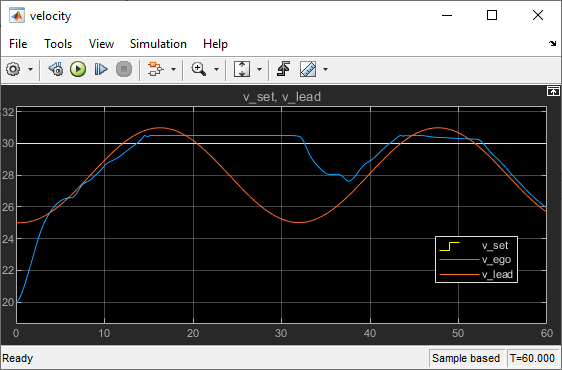
Train Agent Without Constraints

To see the benefit of training an agent with constraint enforcement, you can train the agent without constraints and compare the training results to the constraint enforcement case.

To train the agent without constraints, use the rlACCwithoutConstraint model. This model applies the actions from the agent directly to the environment, and the agent uses the same action and observation specifications.

mdl = 'rlACCwithoutConstraint';
open_system(mdl)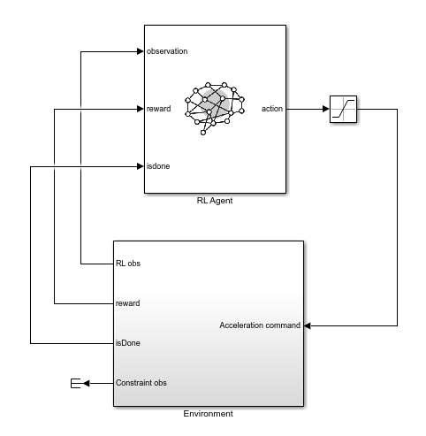

Create an RL environment using this model.

agentblk = [mdl '/RL Agent'];
env = rlSimulinkEnv(mdl,agentblk,obsInfo,actInfo);
env.ResetFcn = @(in)localResetFcn(in);

Create a new DDPG agent to train. This agent has the same configuration as the agent used in the previous training.

agent = createDDPGAgentACC(Ts,obsInfo,actInfo);

Train the agent using the same training options as the in the constraint enforcement case. For this example, as with the previous training, load a pretrained agent. To train the agent yourself, set trainAgent to true.

trainAgent = false;
if trainAgent
    trainingStats2 = train(agent,env,trainingOpts);
else
    load rlAgentACC agent
end

The following figure shows the training results.

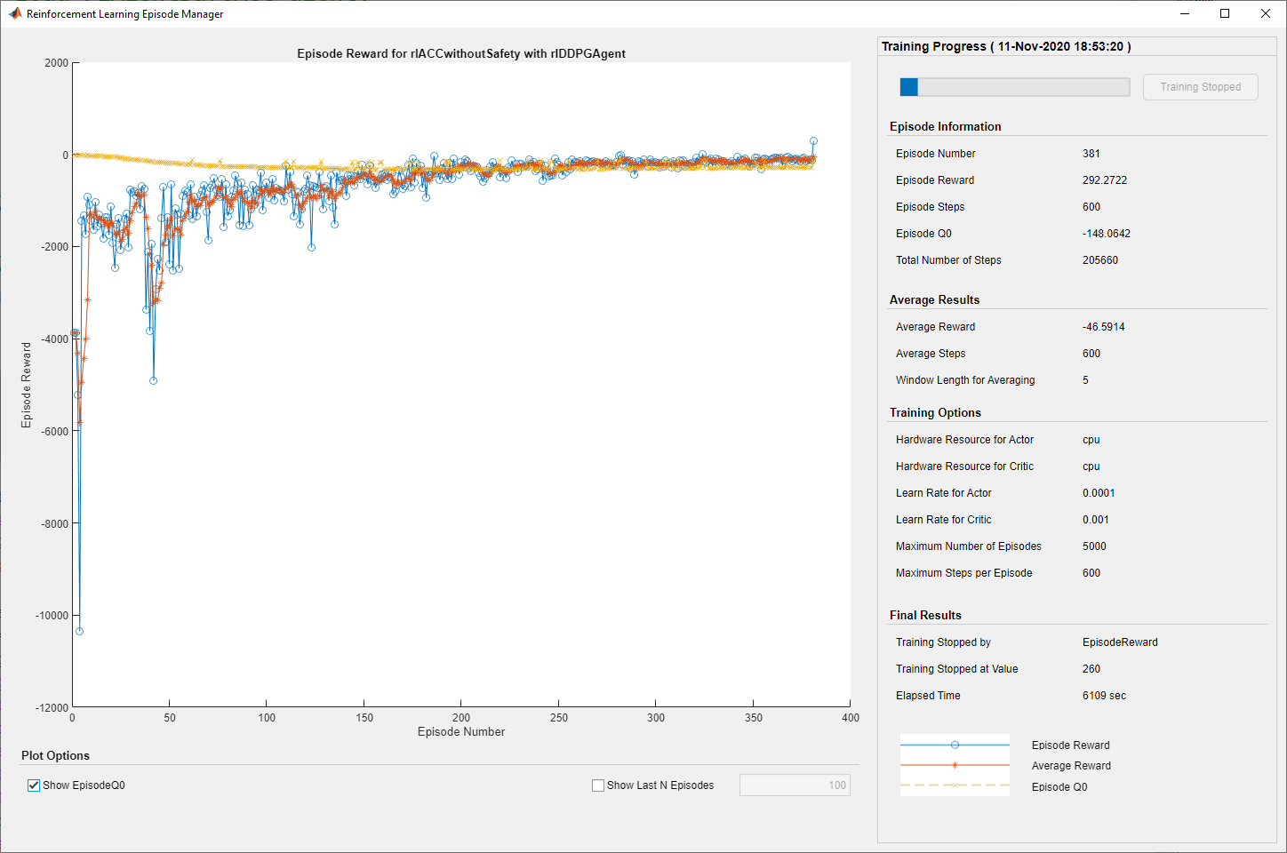
Since Total Number of Steps is less than the product of Episode Number and Episode Steps, the training includes episodes that terminated early due to constraint violations.

Run the trained agent and plot the simulation results.

x0_lead = 80;
sim(mdl)

bdclose('rlLearnConstraintACC')
bdclose('rlACCwithConstraint')
bdclose('rlACCwithoutConstraint')

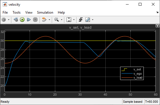
Local Reset Function

function in = localResetFcn(in)
% Reset the initial position of the lead car.
in = setVariable(in,'x0_lead',40+randi(60,1,1));
end